
Ever found yourself staring at a jumbled mess of data in one tiny Excel cell, wishing you could magically split it into neat, organized columns?
Well, guess what? You can! And it’s not magic, it’s just Excel doing what it does best — making our lives easier.
To split cells in Excel:

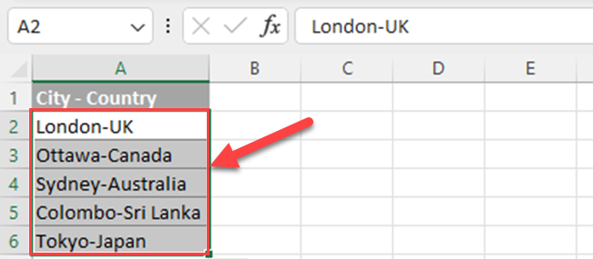
- Select the cells you want to split
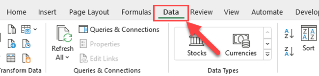
- Navigate to the Data tab
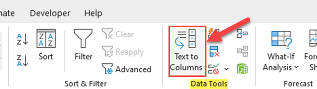
- Click on ‘Text to Columns‘
- Choose the split method
- Click ‘Finish’
In this article, we’ll go over the “Text to Columns” method as well as all of the common ways to split cells in Excel.
Choose the method that suits your data and efficiently manage and organize your Excel spreadsheets.

Let’s get started!
Basic Concepts for Splitting Cells in Excel
Splitting cells in Microsoft Excel is the process of dividing the data within a single cell into multiple cells, either by separating the contents at specific points or by distributing them across multiple columns.
In most cases, this is done when data in a single cell needs to be separated for better readability or analysis.
Excel offers several methods for splitting cells, including the use of the Data tab and built-in functions like Text to Columns.

In the next four sections, we’re going to go over the available methods in depth so that by the end, you can comfortably split cells in Excel in a variety of ways.
1. Using ‘Text to Columns’ to Split Cells
In this section, we’re going to dive into a handy tool available in Excel called Text to Columns. This powerful function is used to split the content of cells based on a specific delimiter or fixed width.
It’s particularly useful when dealing with large datasets, where manual editing would be time-consuming or prone to errors.
1. Access ‘Text to Columns’ Tool
To split cells in Excel effectively, you can use the Text to Columns tool. To access the tool, follow these simple steps:
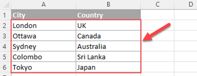
1. Select the cell or column containing the text you want to split.
2. Go to the “Data” tab in the ribbon.
3. In the “Data Tools” group, click “Text to Columns”.
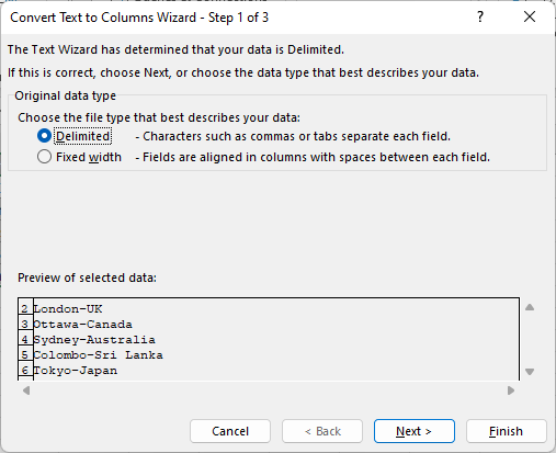
4. The “Convert Text to Columns Wizard” will open, and you can proceed with the desired mode.
2. Delimited Mode
In the Delimited mode, you can split cell text based on a specific delimiter character (comma, space, tab, etc.).
Use the following steps:
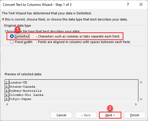
1. Select the “Delimited” option in the wizard, and click “Next”.
2. Choose your delimiter(s):
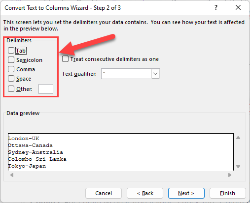
- Tab: To divide text using tabs, check the “Tab” option.
- Semicolon: For semicolon-separated values, check the “Semicolon” option.
- Comma: For comma-separated values, check the “Comma” option.
- Space: To split text using spaces as a delimiter, check the “Space” option.
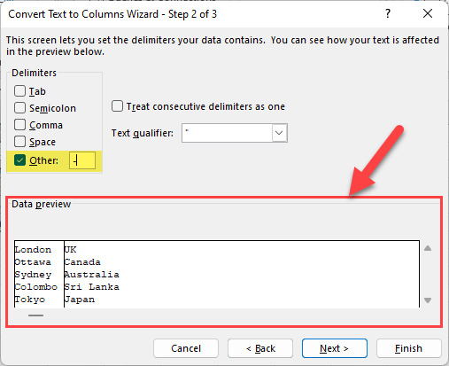
- Other: For a custom delimiter character, check the “Other” option and enter the character in the box.
3. When you select the delimiter, you can preview the data.
4. Click “Finish”.
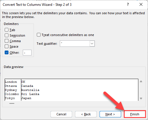
5. Then, Excel will split the data of selected cells into separate columns.

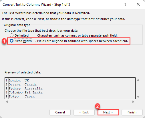
3. Fixed Width Mode
The Fixed Width mode allows you to split cell content by specifying column widths.
Follow these steps to apply this mode:
1. Select the “Fixed Width” option in the wizard, and click “Next”.
2. Create column breaks by clicking at the desired positions on the data preview.
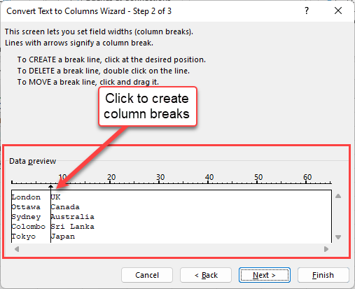
To adjust a break, click and drag it to the desired location. To remove a break, double-click on it.
3. Click “Finish”.
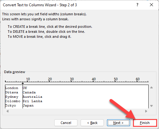
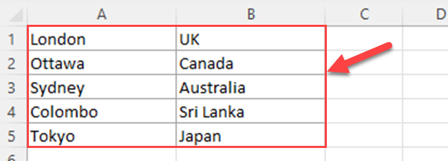
Then, Excel will split the data into column B as below.
If you want to keep the source data, go to step 3 of 3 – “Convert Text to Columns Wizard” and change the destination cell.
By using the appropriate Text to Columns mode, either Delimited or Fixed Width, you can effectively split cells in Excel based on your specific needs.
2. Using Flash Fill to Split Cells
In this section, we’ll explore how to split cells in Excel using the Flash Fill feature.
Flash Fill is a feature in Microsoft Excel that automatically separates or combines data based on patterns it recognizes in your data. Here’s a simple explanation of how to use Flash Fill to split cells:
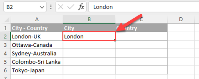
1. Start Flash Fill: In the adjacent empty column (where you want the separated data to appear), type the first split you want Excel to recognize.
2. Once you’ve typed the first split correctly, press “Ctrl + E” on your keyboard, or click the “Flash Fill” button in the “Data” tab of the Excel ribbon.
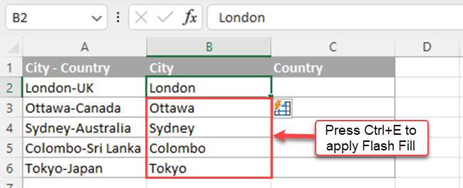
Excel will automatically recognize the pattern and fill in the remaining cells. Make sure to review the results.
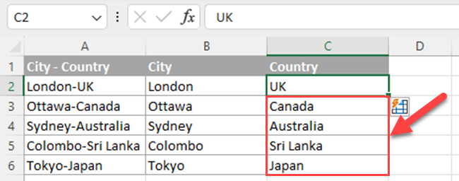
If you have additional data to split, follow the same steps for the other splits you want to do.
That’s it! Excel will automatically apply the Flash Fill feature to recognize patterns and split cells accordingly. Remember that Flash Fill works best when the data has consistent patterns, but you can always review and adjust the results if needed.
3. Using Formulas to Split Cells
In this section, we’ll explore how to split cells in Excel using formulas. There are several functions available in Excel that can help you split the cells effectively.
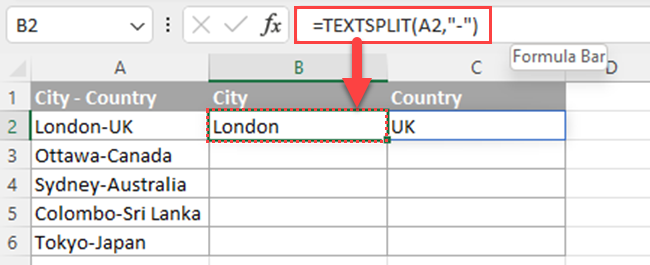
1. TEXTSPLIT Function
The TEXTSPLIT function operates similarly to the Text-to-Columns feature, but it functions as a formula. It helps you to split data into columns or rows.
The syntax of the TEXTSPLIT function is =TEXTSPLIT(text,col_delimiter,[row_delimiter],[ignore_empty], [match_mode], [pad_with]).
You can use the TEXTSPLIT function to split all the data in one cell into two or more cells.

Let’s apply the TEXTSPLIT function to the previous example as below.
Row_delimiter, the third argument, can be used to split cells into separate rows if you’d want.
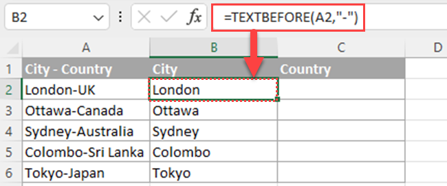
2. TEXTBEFORE and TEXTAFTER Functions
Microsoft recently released two new text functions for splitting cells.
The TEXTBEFORE function gives you the text that comes before a specific character or set of characters in a text.
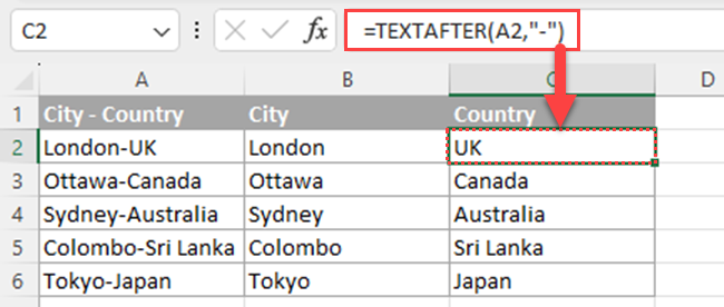
On the other hand, the TEXTAFTER function gives you the text that comes after a specific character or set of characters in a text.
You can use the TEXTBEFORE function to separate the city from the original data in the previous example.
You can also use the TEXTAFTER function to extract data (country) from the first column in that example.
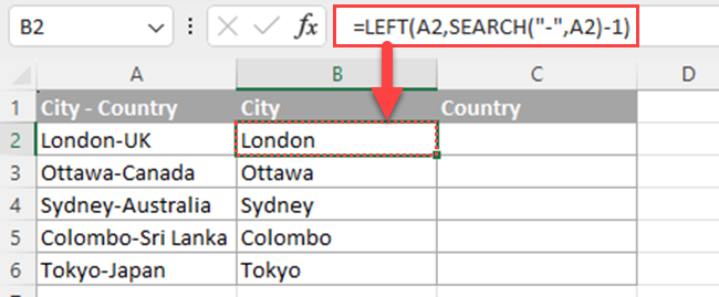
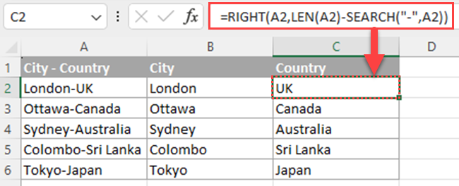
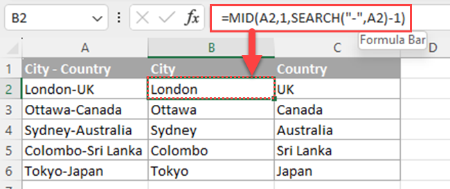
3. LEFT, RIGHT, and MID Functions
If you are not a Microsoft 365 user, the above functions are not available for you. Then, you can use Excel’s LEFT, RIGHT, and MID text functions to split cells.
The LEFT and RIGHT functions in Excel can be used to extract specific characters from the beginning or end of a text string.
The MID function in Excel is used to extract a specific substring from a text string, starting at a specified position.
1. City: =LEFT(A2, SEARCH(“-“, A2) – 1)
2. Country: =RIGHT(A2, LEN(A2) – SEARCH(“-“, A2))
3. City: =MID(A2,1,SEARCH(“-“,A2)-1)
4. Country: =MID(A2,SEARCH(“-“,A2)+1,LEN(A2)-SEARCH(“-“,A2))
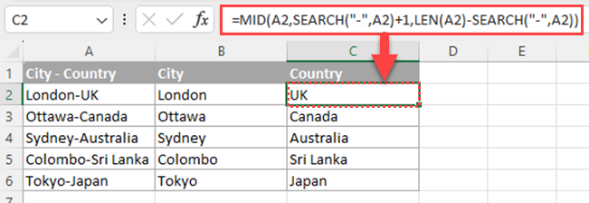
In the above formulas, the SEARCH function is used to find the position of the dash between the city and the country.
The LEN function is used to calculate the total length of the text string.
4. Using Power Query to Split Cells
Power Query is a useful data transformation and visualization tool available in Excel 2013, Excel 2016, Excel 2019, and Excel for Microsoft 365.
It allows you to split data, transform data, and clean data more efficiently.
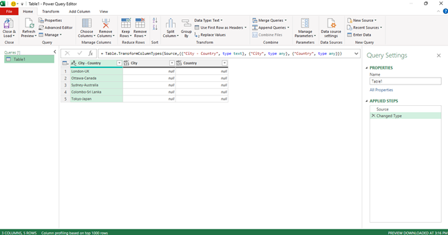
1. Access Power Query Editor
To access the Power Query Editor:
1. Open your Excel workbook containing the data to be processed.
2. Select any cell in your table or range.
3. Click the Data tab (or Power Query tab for Excel 2013 users).
4. Click on the From Table/Range button.
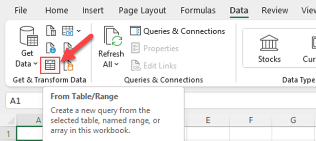
The Power Query Editor will open, displaying a preview of your data.
2. Split a Column into New Columns
In the Power Query Editor, you can split a column into multiple new columns in multiple ways.
For example, you can split the column by a specific delimiter or by fixed-length positions.
Here’s a step-by-step guide on splitting a column by a delimiter:
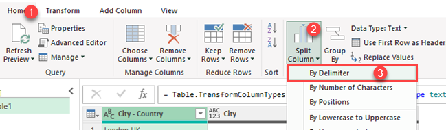
1. Select the column you want to split.
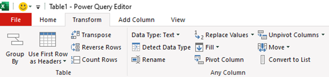
2. Click on the Home tab in the Power Query Editor.
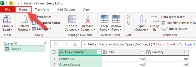
3. Locate the Split Column dropdown menu and choose By Delimiter.
4. Select the appropriate delimiter from the options, and click on OK.
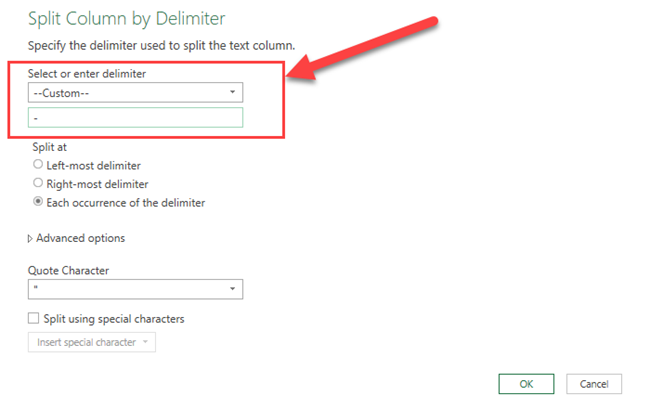
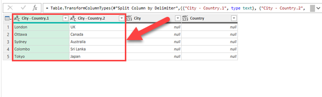
5. The selected column will be split into new columns with a period (.) and a number suffix denoting each split section of the original column.
3. Transform and Clean Data
After splitting your columns, you can further transform and clean your data within the Power Query Editor.
Some common operations include:
- Renaming new columns: Right-click the column header and choose Rename from the context menu.
- Changing data types: Select the column, then click on the Data Type icon in the Transform tab and choose the appropriate data type.
- Replacing values: Select the column, click on the Replace Values option in the Transform tab, and enter the values you want to replace or substitute.
Once your data transformations and cleaning are complete, you can load the data back to your Excel sheet.
Click on the Home tab in the Power Query Editor and choose the Close & Load option. This will add a new sheet to your workbook containing the transformed data.
If you’d like to learn how to split columns by delimiters in Power BI using DAX, watch the video below:
Final Thoughts
Splitting cells in Excel can be done in various ways to manage data efficiently. The “Text to Columns” feature is perfect for splitting data based on a chosen delimiter, such as commas or spaces.
For more control, use formulas like “TEXTSPLIT”, “TEXTBEFORE”, “TEXTAFTER”, “LEFT,” “MID,” or “RIGHT” to extract specific characters from a cell. Combine functions like “SEARCH” and “LEN” to split data based on specific patterns or positions.
When dealing with complex data, the “Flash Fill” feature can be a time-saving option. It automatically recognizes patterns and splits data accordingly.
Additionally, consider using Excel’s array formulas or Power Query for more advanced data-splitting tasks.
Explore these methods based on your data’s characteristics, and with practice, you’ll master the art of cell splitting in Excel, making data manipulation a breeze!
Frequently Asked Questions
How can I divide a cell into multiple rows?
To divide a cell into multiple rows in Excel, you can use the TEXTSPLIT function with its’ third argument (row_delimiter).
What is the method to separate cells horizontally?
To separate cells horizontally in Excel, use the Text to Columns feature. Select the cell or cells you want to split, and then click on the Data tab.
In the Data Tools group, click Text to Columns, and follow the steps in the Convert Text to Columns Wizard.
Which shortcut is used for splitting cells in Excel?
There is no direct shortcut to split cells in Excel. However, you can use shortcuts to access the Text to Columns feature (Alt + A + E) for splitting cells horizontally.
What formula can be used for splitting text in Excel?
To split text in Excel, you can use various formulas like TEXTSPLIT, TEXTBEFORE, TEXTAFTER or LEFT, RIGHT, and MID in combination with FIND or SEARCH functions.
How do I halve a cell in Excel 2020?
To halve a cell in Excel 2020, you can use the “Split” feature with conditional formatting.
First, select the cell you want to halve and apply a gradient fill from the Fill -> Gradient options.
Next, adjust the gradient stops to give the appearance of a split cell or “halved” cell.
What is the technique to separate first and last names in Excel?
To separate first and last names in Excel, use the Text to Columns feature or formulas.
For Text to Columns, select the cell containing the names, go to Data > Text to Columns, and follow the steps in the wizard.
Alternatively, you can use formulas like =TEXRTSPLIT(A1,” “), where A1 contains the full name.


