
Strikethrough in Excel is like drawing a line through words or numbers to show they are changed or deleted, but keeping them visible. It helps you show updates in Excel sheets.
There are many ways for you to apply strikethrough in Excel. You can do this easily by using a special shortcut on your keyboard. This makes it quick and easy for everyone to use, whether they know Excel very well or not.
To apply the Excel Strikethrough shortcut, you must:

- Select the cell where you want to apply the shortcut.
- Press Ctrl + 5. If you are a Mac user, press the Command + Shift + X combination.

To use this feature well, it’s important to learn the shortcuts and to know when to use strikethrough in Excel. This will help you produce better quality and neater sheets.
Learning these shortcuts will help you assemble sheets that clearly show any changes or updates you want to share with others.
What is Excel Strikethrough
Excel strikethrough is a formatting tool that allows you to cross out text within a cell.
This feature is particularly useful for highlighting items that have been completed, invalidated, or are no longer relevant.
Unlike Microsoft Word, there are no strikethrough formatting buttons in Microsoft Excel.
Correspondingly, you must follow a lengthy process to apply the strikethrough format in Excel.

How to Apply Strikethrough Manually
To apply strikethrough in Excel, you must use the Format Cells dialog box.
Follow the steps given below:
Step 1
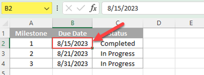
Select the cell where you want to apply the strikethrough format.
For example, if you want to cross out the cell value (the due date) in cell B2, Select cell B2.
Step 2
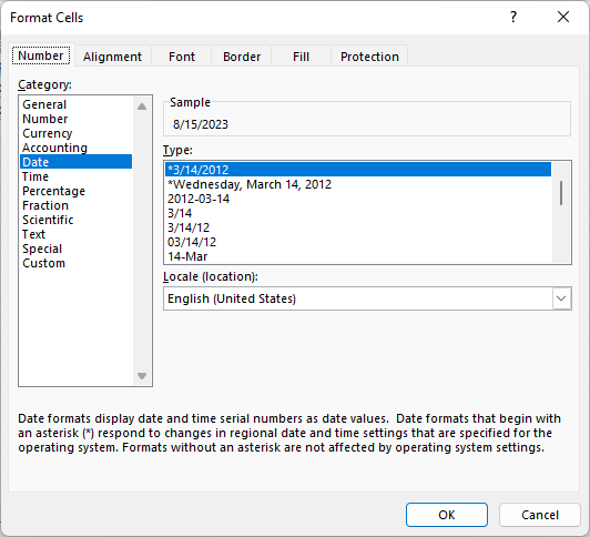
Right-click on the desired cell and click ‘Format Cells’ (or press Ctrl + 1) to open the Format Cells dialog box.
Step 3
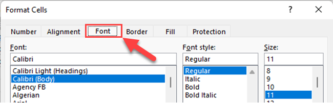
Go to the ‘Font’ tab.
Step 4
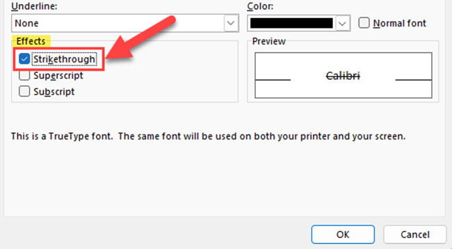
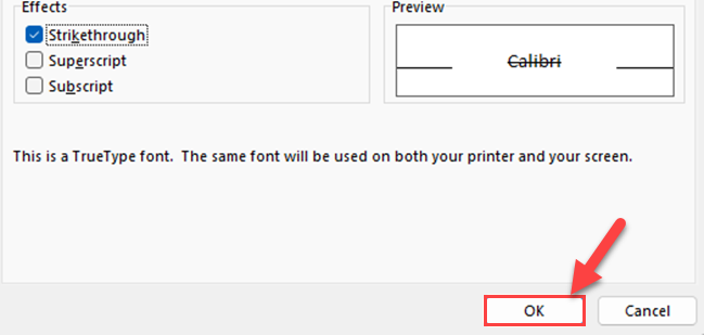
Under ‘Effects’, check the box next to ‘Strikethrough’.
Step 5
Click ‘OK’.
You can remove the strikethrough format by repeating the above steps for applying the strikethrough format, but uncheck the box next to ‘Strikethrough’ in the ‘Format Cells’ dialog box.
It’s essential to know that you can apply strikethrough formatting to an entire cell, a specific part of the cell content, or a range of cells, depending on your needs.

Since there is no button in the Excel Ribbon for the Strikethrough formatting in Excel, it is important to know the shortcut key for Strikethrough Text in Excel.
What is The Shortcut Key for Strikethrough Text in Excel
A quick and convenient way to apply the strikethrough format to a selected cell or text is by using keyboard shortcuts.
In this section, we will cover strikethrough shortcut keys for Windows and Mac users.

1) Strikethrough Text Shortcut Key for Windows Users
If you are a Windows user, to apply strikethrough using keyboard shortcuts, follow the steps below:
Step 1
Select the cell or range of cells that you want to apply the strikethrough to.
For example, if you want to apply the strikethrough option to cell range B2 to B3, select cells as below.
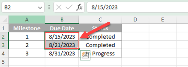
If you need to apply strikethrough to multiple cells that are not adjacent to each other, hold the Ctrl key while selecting the cells.
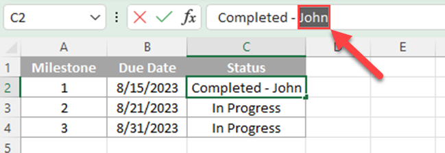
You can also select a specific part of the cell content if you only want to strike through a part of it.
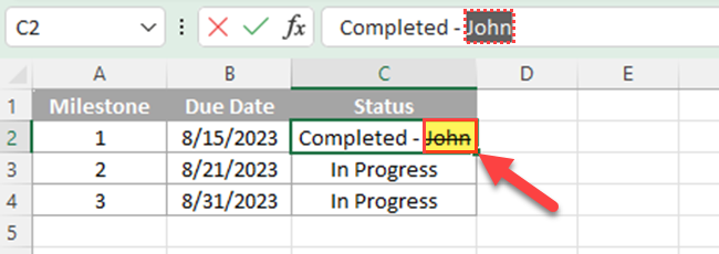
For example, if you want to strike out the name in cell C2, select only that name. To select a part of a text in a cell, double-click and enter the edit mode of that cell.
Step 2
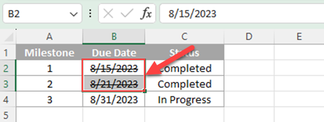
Simply press Ctrl + 5.
If you’ve selected cells, the strikethrough formatting is applied to the entire cell content.
If you’ve selected only a part of the cell content, the strikethrough formatting is applied only to that selected part.
2) Strikethrough Text Shortcut Key for Mac Users
If you are a Mac user, to apply strikethrough using keyboard shortcuts, follow the steps below:
Step 1
Select the cell or range of cells that you want to apply the strikethrough to.
For example, if you want to apply the strikethrough option to cell range B2 to B3, select cells as below.
If you need to apply strikethrough to multiple cells that are not adjacent to each other, hold the Command key while selecting the cells.
You can also select a specific part of the cell content if you only want to strike through a part of it.

For example, if you want to strike out the name in cell C2, select only that name.
Step 2
Simply press Cmd + Shift + X.
If you’ve selected cells, the strikethrough formatting is applied to the entire cell content.
If you’ve selected only a part of the cell content, the strikethrough formatting is applied only to that selected part.
You can see that the strikethrough format doesn’t appear in the formula bar.
The keyboard shortcuts are an efficient and quick way to apply the strikethrough in Excel.
Ctrl+5 for Windows and Command+Shift+X for Mac saves you time and maintain your workflow uninterrupted while keeping your spreadsheet organized and up to date.
How to Add Strikethrough Icon to Quick Access Toolbar?
If you frequently use the strikethrough feature, adding the icon to the Quick Access Toolbar can help you remove strikethrough easily.
The Quick Access Toolbar in Excel can be customized to include the Strikethrough format icon, allowing for a more efficient approach to applying strikethrough formatting to your text.
This method is particularly useful for those who seek a streamlined process in Excel or prefer using their mouse for formatting instead of keyboard shortcuts.
To add the icon, follow the below steps.
Step 1
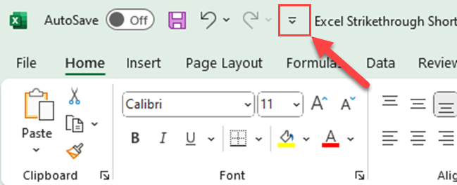
Click on the small dropdown arrow in the QAT located at the top-left corner of the Excel window.
Step 2
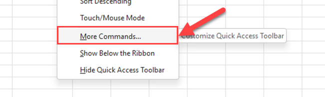
Choose “More Commands…” from the dropdown list.
Step 3
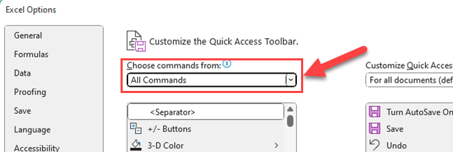
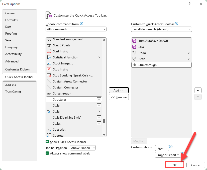
In the “Excel Options” window, select “All Commands” from the “Choose commands from” dropdown.
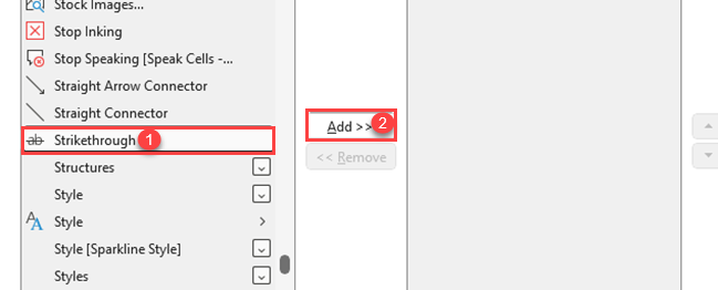
Step 4
Scroll down, select the “Strikethrough” command, and press the “Add >” button to add it to the QAT.
Step 5
Click “OK” to save the setting.
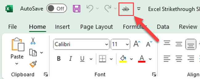
Now, you can simply select the cells containing the strikethrough and click on the Strikethrough icon in the QAT to apply the formatting.
How to Use VBA For Strikethrough
Visual Basic for Applications (VBA) is a useful tool for applying various formatting options in Excel, including the strikethrough feature.
To apply strikethrough formatting using VBA, you can easily create a macro.
Let’s go through the steps of creating and using a simple strikethrough macro:
Step 1
Press Alt + F11 to open the VBA editor in Excel.
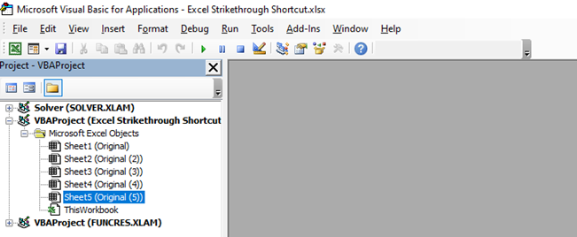
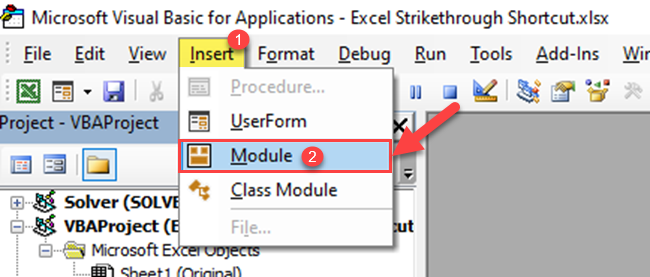
Step 2
Click on Insert from the top menu and choose Module to insert a new module.
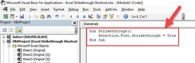
Step 3
In the newly opened module window, copy and paste the following VBA code:
Sub Strikethrough()
    Selection.Font.Strikethrough = True
End Sub
When you run the above macro, the cells you selected will get the strikethrough line on them.
Remember, this VBA code will only work with the currently selected cells, so ensure that you’ve selected the appropriate range before running the macro.
If you like to learn how to dynamically control font properties via DAX, watch the following video:
Final Thoughts
Using the Excel strikethrough is a valuable skill to highlight or mark specific data in your spreadsheet. Being able to quickly apply and remove the strikethrough format saves time and enhances productivity.
In summary, to apply the strikethrough in Excel, you can use Ctrl + 5 on Windows or Cmd + Shift + X on Mac. This shortcut works for single cells, multiple cells, or even specific parts of the data in cells.
Remembering these shortcuts helps you to efficiently use strikethrough in Excel and maintain a clean, professional appearance for your spreadsheets.
By mastering this shortcut, you’ll be well-equipped to handle various data organization and presentation tasks in Excel.
Frequently Asked Questions
In this section, you’ll find some frequently asked questions you may have when using the Excel strikethrough format shortcut.

What is the keyboard shortcut for strikethrough in Excel?
The keyboard shortcut for strikethrough in Excel is Ctrl + 5 (for Windows) or Command + Shift + X (for Mac).
To apply the effect, hold the appropriate keys, and the selected cell content will have a line crossing it.
How to apply strikethrough using shortcuts in Excel Online?
Unfortunately, Excel Online does not support the same keyboard shortcuts as the desktop version. There isn’t a specific shortcut for strikethrough in Excel Online.
However, you can apply the strikethrough formatting by opening the Format cells dialog box and adjusting the settings from there.
What is the strikethrough shortcut for Microsoft Word and Outlook?
In MS Word and Outlook, the keyboard shortcut for applying a strikethrough is Ctrl + D (Windows) or Command + D (Mac).
This opens the Font dialog box, where you can check the Strikethrough option.
How can I conditionally apply strikethrough formatting in Excel?
To conditionally apply strikethrough formatting in Excel, use Conditional Formatting with custom formula rules.
For example, if you’d like the strikethrough effect on values less than a specific threshold, create a rule that formats cells accordingly, and then apply it to the desired range.
What is the shortcut for strikethrough in Google Sheets and Docs?
The keyboard shortcut for strikethrough in Google Sheets and Google Docs is Alt + Shift + 5 (Windows) or Command + Shift + X (Mac).
This combination will add a line crossing the selected text in the respective applications.
How to cross out a cell diagonally in Excel?
Crossing out a cell diagonally is not a built-in formatting feature in Excel. To achieve this effect, you can insert a shape – specifically a diagonal line – over the targeted cell.
Go to the Insert tab, click Shapes, and choose the line type that matches the desired diagonal direction, then draw it over the cell. Resize and align the line to create the appearance of a diagonal cross-out.


