
Excel is a powerful tool that helps you store data, perform calculations, and organize information. To make the best use of the tool, you need a quick reference to guide you through the various functions, commands, and shortcuts.
This article is a comprehensive Excel cheat sheet specifically designed for beginners. It starts with the basics and moves on to functions, formulas, and data analysis tools.
Mark sure to bookmark this page so you can find it easily in a pinch or if you’d like to download and print the cheat sheet, you can do it below.

Let’s get started!
Cheat Sheet for Navigating the Excel Interface
We start with a cheat sheet for navigating the Excel interface, which can seem a little intimidating at first glance, but don’t worry!
This section will give you the lowdown on the essential features, shortcuts, and tricks, including the ribbon, workbooks and worksheets, and rows, columns, and cells.
1. Ribbon
The ribbon is at the top of your screen. Each tab includes a set of commands to help you perform tasks quickly
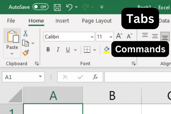
To show or hide the ribbon commands, press Ctrl-F1.
If you can’t remember the location of a command, you can always use the search bar on the ribbon to find it.

2. Workbook and Worksheets
A workbook is an Excel file that contains one or more worksheets. Worksheets are where you organize and process your data.
You can navigate through your worksheets using keyboard shortcuts:
Press Ctrl + Page Up to move to the next sheet.
Press Ctrl + Page Down to move to the previous sheet.
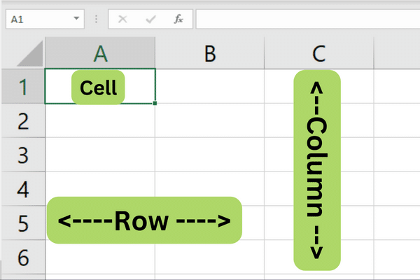
3. Rows, Columns, and Cells
Worksheets are made up of rows, columns, and cells.
Rows are labeled with numbers, and columns are labeled with letters. Cells are the intersection of rows and columns and are referred to by their column and row labels, like A1 or B2.
To navigate within a worksheet, use the arrow keys to move up, down, left, or right.
You can also use the following shortcuts:
Ctrl + up arrow
Ctrl + down arrow
Ctrl + left arrow
Ctrl + right arrow
To select a range of cells, click and drag with your mouse or hold the Shift key while using the arrow keys.
To quickly select the entire row or column, click on the row number or column letter.
Now that you know how to navigate the Excel interface, let’s go over some of the basics of the program in the next section of our cheat sheet.
Cheat Sheet for Excel Basics
This section of the cheat sheet features the foundations you need for working with data in your spreadsheets, such as how to enter, edit, move, and find data.
1. Entering Data
To enter data in Excel, simply click on a cell and start typing. Press ‘Enter’ or ‘Tab’ to move to the next cell in the row or column, respectively.
You can also use the arrow keys to navigate between cells.
2. Editing Data
To edit data in a cell, double-click on the cell or press ‘F2’ to edit the cell contents directly.
You can also click on the cell and edit the content in the formula bar located at the top of the Excel window.
Press ‘Enter’ to apply your changes.
To undo, press ‘Ctrl’ + ‘Z’, or use the ‘Undo’ button in the Quick Access Toolbar.
To redo, press ‘Ctrl’ + ‘Y’, or use the ‘Redo’ button in the Quick Access Toolbar.
3. Moving And Selecting Data
To move a single cell or a range of cells, follow these steps:

Click on the cell or cells you want to move.
Hover your cursor over the edge of the cells until it becomes a four-sided arrow.
Click and drag the cells to their new location.
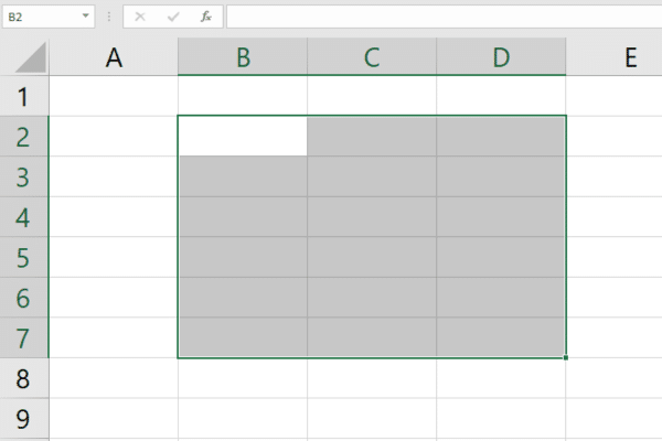
To select a range of cells, click the top-left corner of the range and drag your cursor to the bottom-right corner.
Alternatively, you can use the ‘Shift’ + arrow keys to select cells.
To select non-adjacent cells, hold down ‘Ctrl’ while clicking the desired cells.
4. Find and Replace
To find a specific value or text in your worksheet:
Press ‘Ctrl’ + ‘F’ to open the ‘Find’ dialog box.
Enter your search query.
Click ‘Find Next’ or ‘Find All’ to locate the instances of your search term.
To replace a value or text:
Press ‘Ctrl’ + ‘H’ to open the ‘Replace’ dialog box.
Enter the value you want to find in the ‘Find what’ field.
Enter the value you want to replace within the ‘Replace with’ field.
You can now click ‘Replace’ to replace a single instance, or ‘Replace All’ to replace all instances in the selected range or the entire worksheet.
With the basics done, let’s take a look at what you need to remember when formatting cells in the next section.
Cheat Sheet for Formatting Cells
When entering dates or times, format the cells accordingly before inputting the data.
To format a cell:
Right-click on the cell.
Choose ‘Format Cells’.
Select the desired format.
1. Number Formats
You can choose the appropriate number format to simplify data presentation. Here’s how you can apply different number formats:
Select the cells you want to format.
Right-click and choose ‘Format Cells’ or use the shortcut Ctrl+1.
Click on the ‘Number’ tab, and select the desired format from the list.
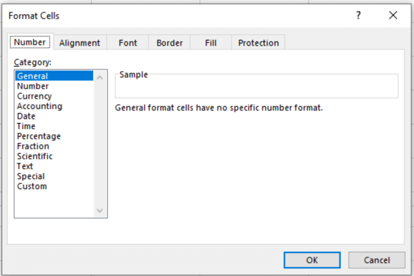
Common number formats include:
General: Default format without specific styles.
Number: Displays numbers with decimals and commas.
Currency: Adds currency symbols to the numbers.
Percentage: Represents the value as a percentage.
Date: Formats the cell value as a date.
2. Text Formats
Enhance the readability of your text by applying various formatting options.
When you select the cells containing the text you want to format, you can use keyboard shortcuts for quick formatting:
Ctrl+B for bold.
Ctrl+I for italic.
Ctrl+U for underline.
Alternatively, use the toolbar options in the ‘Home’ tab, like ‘Font’ and ‘Alignment’.
3. Borders And Shading
Apply borders and shading to emphasize or differentiate cell data. Follow these steps:
Select the cells you want to format.
Right-click and select ‘Format Cells’, or use the shortcut Ctrl+1.
Click the ‘Border’ tab to customize cell borders or the ‘Fill’ tab for shading.
4. Conditional Formatting
Conditional formatting allows you to apply formats based on specific conditions. Here’s how to implement it:
Select the cells you want to apply conditional formatting to.
Click on the ‘Home’ tab and choose ‘Conditional Formatting’ from the ribbon.
Select from the list of available conditions or create a new rule.
Assign the appropriate format for the selected condition.
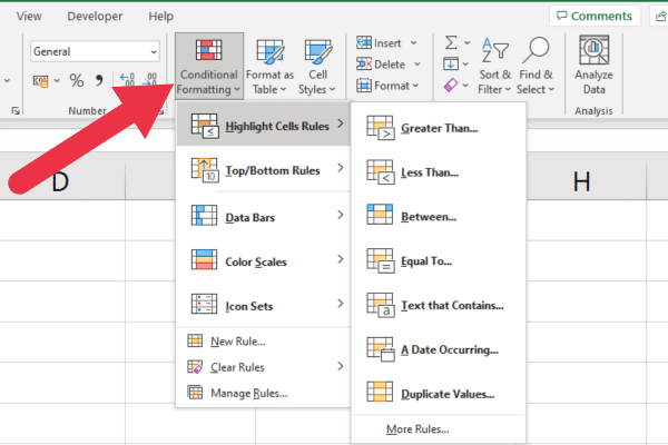
This powerful tool can help you identify trends, inconsistencies, or specific values in your spreadsheet with ease.
In the next section of our reference guide, we provide a cheat sheet for popular Excel formulas. Let’s go!
Excel Formulas Cheat Sheet
Before we give you the most commonly used Excel formulas and functions, here is a quick primer on how to use them.
Formulas in Excel are used to perform calculations and manipulate data with built-in functions.

To create a formula, start with an equal sign (=) followed by a combination of numbers, cell references, and mathematical operators.
Here is an example that adds the values in the range A1 to A5
=SUM(A1:A5)
With that in mind, let’s look at some basic Excel formulas and functions.
1. Excel Text Functions
Sometimes you need to chop up strings in a cell. For example, extracting the parts of an address is a common task. These text functions are very useful:
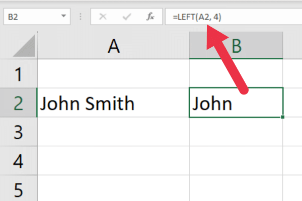
LEFT: this function returns the first or multiple characters from a string.
RIGHT: gets the last or multiple characters from a string.
MID: gets characters in the middle of the string.
CONCAT: puts strings together.
This example shows the use of the LEFT function to extract the first four characters:
The find functions provide powerful features for working with text:
FIND: locates a specific string within another text string
SEARCH: similar to FIND but works with wildcard characters
In the next section, we take a look at some popular Excel math functions.
2. Excel Math Functions
There is a long list of Excel functions that includes some highly complex computations. Here are the ones you will most commonly use:
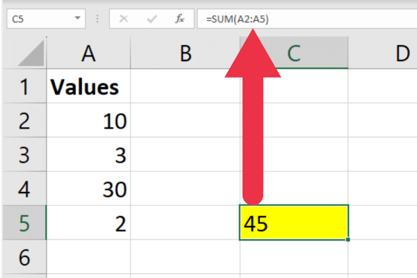
SUM: Adds up a range of numbers.
AVERAGE: Calculates the average (arithmetic mean) of a range of numbers.
MIN: Returns the smallest value in a dataset.
MAX: Returns the largest value in a dataset.
COUNT: Counts the number of cells containing numbers within a range.
PRODUCT: Multiplies a range of numbers together.
Here is an example of the SUM function:
3. Excel Time Functions
Time functions help you manage, convert, and manipulate time data.
NOW: Returns the current date and time.
TODAY: Returns the current date without the time.
HOUR: Extracts the hour from a given time.
MINUTE: Extracts the minutes from a given time.
SECOND: Extracts the seconds from a given time.
TIME: Constructs a time value from separate hour, minute, and second values.
4. Excel Lookup Functions
A lookup function searches for specific values within a range or table and returns corresponding data from another column or row. These are the most common for Excel users:
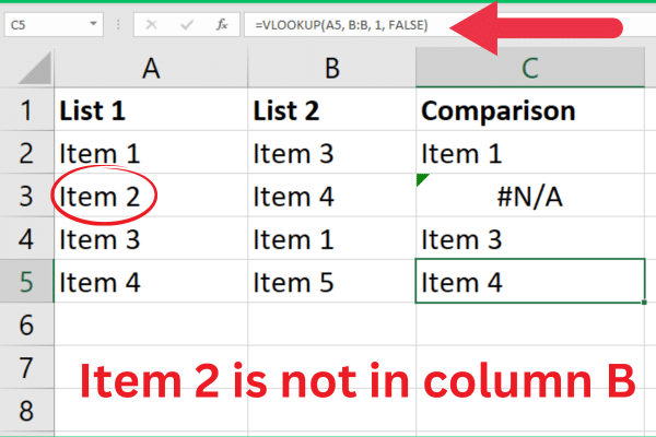
VLOOKUP: Searches for a value in the first column of a table and returns a value in the same row from a specified column.
HLOOKUP: Searches for a value in the first row of a table and returns a value from a specified row in the same column.
INDEX: Returns a value from a specified row and column within a given range or table.
MATCH: Searches for a specified item in a range or array and returns the relative position of the item within that range.
If you’ve got the latest version of MS Excel, there are some new features like XLOOKUP, which is faster than the older functions.
Here’s an example of using the VLOOKUP function:
Cell Referencing with Excel Formulas
Cell referencing is a way to point to a specific cell or range of cells in a formula. There are two types of cell references: absolute and relative.
Absolute refers to a specific cell or range and keeps the same reference even when the formula is copied. It uses a dollar sign ($) to denote absolute referencing, like $A$1.
A relative reference changes when the formula is copied to another cell or range, adjusting the reference based on the new location.
Formula Error Troubleshooting
Formulas can sometimes result in errors due to incorrect syntax, invalid references, or other issues with calculation. Some common error messages are:
#DIV/0!: Division by zero
#NAME?: Occurs when Excel doesn’t recognize text in the formula
#REF!: Invalid cell reference
#VALUE!: Occurs when the wrong data type is used in a formula
To fix errors, check the formula’s syntax, cell references, and data types to make sure they are correct and compatible.
With formulas done, the next section of our reference is for Excel data analysis tools.
Cheat Sheet for Excel Data Analysis Tools
Excel provides a wide range of tools to help you analyze and organize your data effectively. Let’s discuss the various tools and their importance.
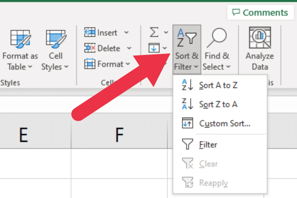
1. Sorting and Filtering
Sorting and filtering in Microsoft Excel enables you to arrange your data in a more organized way. To access the feature:
Go to the Home tab.
Click on “Sort & Filter” in the Editing section.
Choose one of the options in the drop-down list.
These are your options:
Sort A to Z: Orders text data alphabetically or numerical data from the lowest value to the highest.
Sort Z to A: Orders text data in reverse alphabetical order or numerical data from the highest value to the lowest.
Custom Sort: Apply multiple sorting conditions to your data.
Filter: Display only rows that meet specific criteria.
2. Pivot Tables
Pivot tables are used to summarize and consolidate your data effectively. They enable you to perform quick data analysis by dragging and dropping different fields into rows or columns and applying calculations such as sum, average, and standard deviation.
To create a pivot table:
Select your data range.
Click on the ‘Insert’ tab in the Excel toolbar.
Choose ‘PivotTable’ from the drop-down menu and configure your pivot table settings.
Drag and drop fields into rows, columns, and values areas to analyze your data.
3. Charts and Graphs
Visual representations of your data using charts
and graphs can help you gain better insights and make informed decisions. Excel comes with a handy variety of charts and graphs to choose from, including:
Column charts: Compare different data sets across distinct categories.
Bar charts: Display comparisons among discrete categories horizontally.
Line charts: Show trends and patterns over time.
Pie charts: Illustrate proportional data and percentages.
To create a chart in Excel:
Select your data range.
Click on the ‘Insert’ tab in the Excel toolbar and choose desired chart type.
Customize your chart’s design, layout, and formatting to meet your requirements.
Charts and graphs are powerful tools. If you want to see some in action, check out this video:
We’ve covered a lot of ground so far! Up next is a reference for popular Excel keyboard shortcuts.
Cheat Sheet for Excel Keyboard Shortcuts
There are four categories of keyboard shortcuts in Excel:
General Shortcuts
Navigation Shortcuts
Formatting Shortcuts
Data Analysis Shortcuts
1. General Shortcuts
Here are some commonly used shortcuts for routine tasks and Excel commands:
Ctrl + N: Create a new workbook
Ctrl + O: Open an existing workbook
Ctrl + S: Save the current workbook
Ctrl + Z: Undo the last action
Ctrl + Y: Redo the last action
Ctrl + C: Copy the selected cells
Ctrl + X: Cut the selected cells
Ctrl + V: Paste the copied or cut cells
2. Navigation Shortcuts
To navigate within a workbook, try the following shortcuts:
Ctrl + arrow keys: Move to the edge of the current data region
Ctrl + G: Open the Go To dialog box
Ctrl + Page Up: Move to the previous sheet in the workbook
Ctrl + Page Down: Move to the next sheet in the workbook
Ctrl + Home: Move to the first cell in the worksheet (A1)
3. Formatting Shortcuts
Use these shortcuts for formatting in Excel:
Ctrl + 1: Open the Format Cells dialog box
Ctrl + B: Apply or remove bold formatting
Ctrl + I: Apply or remove italic formatting
Ctrl + U: Apply or remove underline formatting
Ctrl + 5: Apply or remove strikethrough formatting
Alt + H + H: Access the Fill Color options
Alt + H + B: Access the Border options
4. Data Analysis Shortcuts
When working with data, these shortcuts can be helpful:
Alt + A + S + S: Sort selected data alphabetically
Alt + A + T: Add or remove a filter to the selected range
Ctrl + Shift + L: Enable or disable AutoFilter
Alt + =: Insert an AutoSum formula
F2: Edit an active cell
Ctrl + Shift + Enter: Enter a formula as an array formula
By mastering these keyboard shortcuts, you can navigate, format, and analyze your data more efficiently and effectively.
Final Thoughts
And there we have it. We’ve covered a lot of ground in this cheat sheet, diving into the essentials of navigating the Excel interface.
This guide is here to simplify your journey with Excel, offering you the key tools, shortcuts, and techniques at your fingertips, so make sure to save it for future reference!
While there’s still a lot more to Excel, mastering these basics will put you on the fast track to becoming an Excel pro. So, keep practicing, keep exploring, and you’ll continue to uncover the immense capabilities that Excel has to offer. Happy spreadsheeting!


