
There are times when you work with data that is not formatted in the way you need. For example, you may have a mix of numbers and text in a cell, and you need to clean up this data.
There are several techniques to remove numbers in Excel from the left of the text. Some methods work when the data has a consistent pattern. VBA or more complex formulas work on less structured data.
This article demonstrates seven methods to delete numbers on the left of text data. By the end, you will have a comprehensive understanding of the different techniques and when to use them.

Let’s go!
How to Use Flash Fill to Remove Numbers in Excel From the Left
Flash Fill is an Excel feature that can automatically fill in patterns for you. It’s a quick and easy way to remove numbers from the left side of cells.
This method may not always work perfectly, but it can be helpful for simple cases. Follow these steps to use Flash Fill:
In an empty column adjacent to your data, type the desired result without the numbers (e.g., if “1234apple” is in cell A1, type “apple” in cell B1).
Select the cell with the new data (B1 in our example) and click the Data tab on the ribbon.
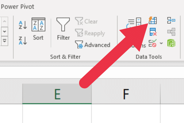
Click the Flash Fill button in the Data Tools section.
Excel will automatically apply the pattern to remove numbers from the left side of the adjacent cells.
This is the location of the Flash Fill button in the Data tab.
If you prefer to use shortcuts, press CTRL + E on Windows or CMD + E on a Mac.
Flash Fill is a handy feature, but as with most things in Excel, there are multiple ways to accomplish the same task.

In the next section, we take a look at how you can do the same thing using the “Text to Columns” feature.
How to Use the Text to Columns Feature to Remove Numbers
You can use the “Text to Columns” feature in Excel to separate numbers from the left of a cell. However, this method assumes that there’s a consistent pattern or delimiter between the numbers and the text in the cell.
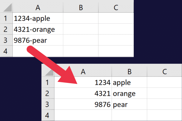
Let’s work with a set of data that uses a dash to separate numbers from letters like this:
1234-apple
4321-orange
9876-pear
This is the before-and-after we want to achieve:
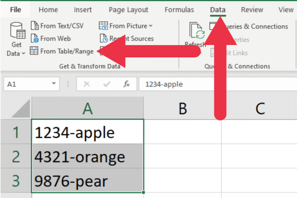
Here’s a step-by-step guide with this sample data set:
Select column A.
Go to the Data tab and click on the Text to Columns wizard.
Choose the Delimited option and click Next.
Uncheck all delimiters (the tab may be applied by default).
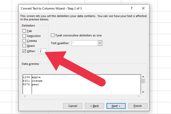
Check the Other delimiter and type “-“ into the input box.
Select the appropriate delimiter (space, comma, etc.).
Click Next and Finish.
The data will now be separated into two columns. The removed characters are in the first column while the rest of the text is in the second column. This picture shows how to set the delimiter:
Next, let’s take a look at five text functions for removing numbers in Excel.
5 Text Functions to Remove Numbers in Excel From the Left
If you know how many characters make up the digits, then you can use a text function to remove them.
Suppose cell A1 contains the string “1234apple”. The first four characters are numbers that we want to remove.
There are several functions that can be used on their own or combined for removing characters that are numeric values.
1. MID Function
You can use the MID function to extract the part of the string that starts from the 5th character.
The MID function extracts a specific section of a text string, given the starting position and the number of characters to extract. The syntax for the MID function is:
MID(text, start_num, num_chars)
text: The text string containing the characters you want to extract.
start_num: The position of the first character you want to extract.
num_chars: The number of characters to extract from the text string.
To remove the numbers on the left, follow these steps:
select cell B2 to contain the function and results.
Type the formula: MID(A1, 5, 7)
The above formula will remove characters from the 5th slot in the string.

2. Combine with the LEN Function
One drawback with this method is that your text string may not always be the same length.
You can use the LEN function to calculate the length dynamically. This function returns the length of a text string.
You can modify the formula to replace the third parameter with the LEN function like this:
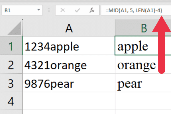
=MID(A1, 5, LEN(A1)-4)
You can copy the formula down by using the fill handle. This picture shows the above formula in use:
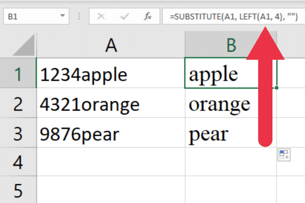
3. Combining LEFT and SUBSTITUTE Functions
The LEFT function returns the leftmost characters from a text string. For example, LEFT(“1234apple”, 4) would return the value “1234”.
This is useful when you want to extract the numbers. But what if you want to remove them?
You can combine LEFT with the SUBSTITUTE function to replace the number with an empty string. This is the format for our example:
=SUBSTITUTE(A1, LEFT(A1, 4), “”)
4. Using the RIGHT and LEN Function
The RIGHT function returns the rightmost characters from a text string. The syntax for the RIGHT function is:
RIGHT(text, [num_chars])
text: The text string containing the characters you want to extract.
num_chars: (Optional) The number of characters to extract from the right side of the text string. If omitted, it defaults to 1.
For example, RIGHT(“1234apple”, 5) would return the value “apple”.
You can also combine the RIGHT and LEN functions to avoid hard coding the number of alpha characters. This is assuming that you know the number of numeric characters.
The format for our example is: =RIGHT(A1, LEN(A1)-4)
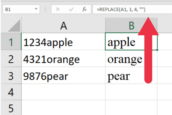
5. Using the REPLACE Function
The REPLACE function can be used to replace a specific number of characters from the left in a cell. This is the syntax:
REPLACE(old_text, start_num, num_chars, new_text)
old_text: the original text string that you want to modify.
start_num: the position in the old_text where you want to start replacing characters.
num_chars: the number of characters in the old_text that you want to replace.
new_text: the text string you want to replace the specified characters with.
The following formula is for our sample data:
=REPLACE(A1, 1, 4, “”)
And that’s the last of our five text functions for removing characters from the left in Excel.
In most cases, the seven methods we’ve covered so far should be enough, but if you want more power, Power Query is the answer, and that’s what we’ll talk about in the next section!

How to Use Power Query to Remove Numbers From Left
Power Query is a powerful data transformation tool available in Excel. The method shown in this section assumes that there is a delimiter between the numbers and the text in the cell.
The first step is to transform the target data into a table:
Go to the Data tab.
Select the cell range.
Choose “From Table/Range” from the Get Data section in the ribbon.
When the Power Query Editor opens, follow these steps:
Select the target column(s).
Go to the “Transform” tab
Click on “Extract” in the ribbon, and choose “Text After Delimiter.”
In the “Text After Delimiter” dialog box, enter a dash (-).
Click “OK” to accept the details.
The transformed column will now have the numbers removed from the left of the text.
Click “Close & Load” to load the transformed data back into your worksheet.
If you’re new to this data tool, check out our tutorial on how to use Power Query in Excel.
If you want to dive deeper into using tables in Power Query, this video walks through some more complex examples:
3 Advanced Techniques Regardless of How Many Characters
The main drawback of the methods so far is that the numbers in all the cells must follow the same pattern or be a specific number of characters.
What if you want to delete characters without a clear pattern in the original data? The techniques in this section are for intermediate Excel users.
1. Combine a Helper Column With a Formula to Remove Characters From Left Of Cells
You can combine functions with helper columns when you don’t know the total length of the numbers. This method requires a two-step process:
use a formula to create a temporary modified version of the original text
use another formula to remove the numbers based on the modified text.
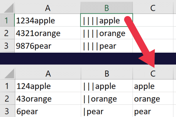
The first step is to use the following formula to replace all the numbers with a specific character (e.g., “|”):
=SUBSTITUTE(SUBSTITUTE(SUBSTITUTE(SUBSTITUTE(SUBSTITUTE(SUBSTITUTE(SUBSTITUTE(SUBSTITUTE(SUBSTITUTE(SUBSTITUTE(A1, “0”, “|”), “1”, “|”), “2”, “|”), “3”, “|”), “4”, “|”), “5”, “|”), “6”, “|”), “7”, “|”), “8”, “|”), “9”, “|”)
The second step is to use the following formula in another helper column (e.g. column C):
=TRIM(RIGHT(SUBSTITUTE(B1, “|”, REPT(” “, LEN(B1))), LEN(B1)))
This is the before-and-after with the formulas in column B and C:
When you start combining functions like this, you can run into issues with choosing the wrong options in your formulas. Our article on how to find circular references in Excel will help you troubleshoot a common error.
You may also want to share a spreadsheet that contains helper columns. It’s important that your colleagues don’t delete or amend the formulas in the intermediate results. Our article on ways to lock columns in Excel will help you to produce the functionality.
2. Create a VBA Macro to Remove Numbers
VBA is a versatile scripting language that lets you automate tasks and create custom solutions within Excel.
For example, you can write a macro that removes numbers from the left of all cells in a specific column or range.
To do so, follow these steps:
Press ALT + F11 to open the VBA editor.
Click Insert > Module to create a new module.
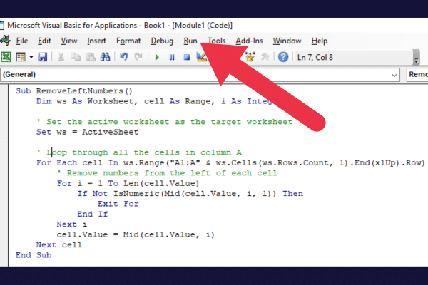
Copy and paste the following code to remove only numbers from the left of column A:
Sub RemoveLeftNumbers()
    Dim ws As Worksheet, cell As Range, i As Integer

    ' Set the active worksheet as the target worksheet
    Set ws = ActiveSheet

    ' Loop through all the cells in column A
    For Each cell In ws.Range("A1:A" & ws.Cells(ws.Rows.Count, 1).End(xlUp).Row)
        ' Remove numbers from the left of each cell
        For i = 1 To Len(cell.Value)
            If Not IsNumeric(Mid(cell.Value, i, 1)) Then
                Exit For
            End If
        Next i
        cell.Value = Mid(cell.Value, i)
    Next cell
End Sub
The last step is to run the macro. Click the green triangle or the “run” menu item.
3. Create a User-Defined Function
You can also create a user-defined function with VBA that you can utilize in your formulas.
To do so, follow these steps:
Press ALT + F11 to open the VBA editor.
Click Insert > Module to create a new module.
Copy and paste the following code:
Public Function RemoveNumbersFromLeft (text As String) As String
    Dim i As Integer
    For i = 1 To Len(text)
        If Not IsNumeric(Mid(text, i, 1)) Then
            Exit For
        End If
    Next i
    RemoveNumbersFromLeft = Mid(text, i)
End Function
Now, return to your Excel sheet and use the public function in a formula.
For example, this formula works by accepting the A1 cell:
=RemoveNumbersFromLeft(A1)
Final Thoughts
In this article, we have explored multiple methods to remove numbers from the left side of text strings in Excel. Each technique has its own advantages and limitations.
No single method is perfect for every situation, but there is sure to be an approach that best suits your needs. With practice, you will become proficient in applying these techniques to handle any data formatting challenge that comes your way.
So there you have it, the ins and outs of removing unwanted digits from the left in Excel. It might look a bit tricky at first, but with the right techniques, you’ll be bossing it in no time! Happy number-crunching!


