
Microsoft Excel, part of the Microsoft Office suite, is a powerful spreadsheet program introduced in 1985 as a competitor to the dominant spreadsheet software at the time, Lotus 1-2-3.
Over the years, Microsoft Excel has become the go-to software program for businesses and individuals, offering a wide range of features for data analysis, visualization, and organization. It is widely used across various industries, such as finance, marketing, human resources, and project management, among others.
This comprehensive guide will provide an in-depth look at Microsoft Excel’s features and functions, from basic operations to advanced capabilities, such as creating charts, PivotTables, and macros. We’ll also include tips and resources for mastering Excel and improving productivity. Is it wrong to say, “It’s time for you to Excel at Excel”?

Either way, let’s get started!
Getting Started with Microsoft Excel
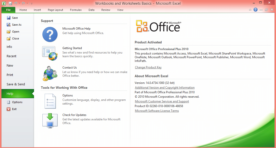
To get started with Microsoft Excel, you will first need to download and install the program on your computer.
Microsoft Excel can be installed as part of the Microsoft Office suite or as a standalone application. You can purchase a subscription to Office 365 or a one-time license for Office 2019. To install Excel, follow the steps provided on the official Microsoft Office website.
After installing Excel, open the program by double-clicking its icon on your desktop or searching for it in the Start menu (Windows) or Launchpad (macOS).
Excel Versions and Availability
Microsoft Excel has evolved over the years to meet the needs of users in a rapidly changing technological landscape. Today, there are different versions of the spreadsheet program available on various platforms, including desktop, online, and mobile, providing users with the flexibility to access and work with their data anywhere and anytime.
In this section we will provide an overview of Excel’s different versions and their availability, highlighting the key features and differences among them.

Let’s start with the desktop version.
Desktop Version
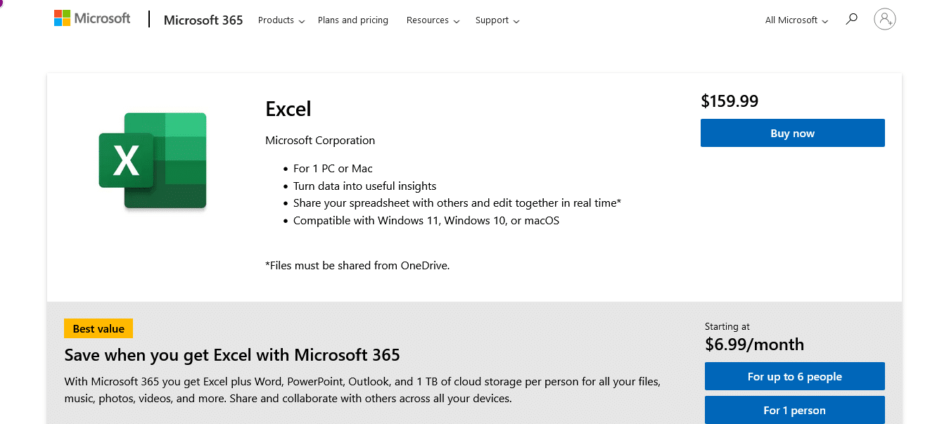
The desktop version of Microsoft Excel is the traditional, feature-rich application installed on Windows and macOS computers. It offers the most comprehensive set of tools and functions for data analysis, visualization, and automation.
It’s available through the Microsoft 365 subscription or as a standalone product, with regular updates and enhancements to improve performance and add new features.
You’ll find it available on:
Microsoft Windows: Excel for Microsoft Windows is the most widely used version and offers the most extensive range of features and capabilities.
macOS: Excel for macOS provides similar functionality to the Windows version, with some differences in keyboard shortcuts, layout, and specific features.
Don’t want to download anything, we get it, the web version is what you need.
Web Version
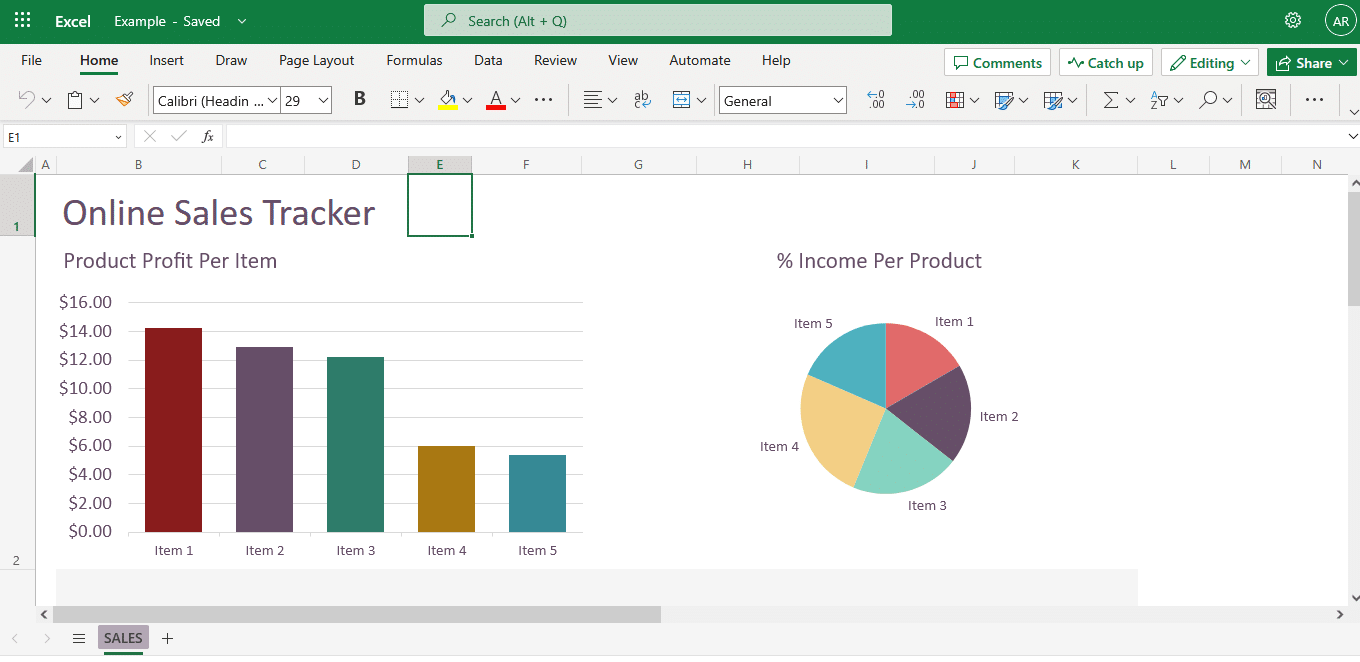
For users seeking a cloud-based solution or those without access to the full desktop version, the web version of Microsoft Excel is available as part of Microsoft 365. MS Excel Online is a web-based version of Excel accessible through a web browser, allowing users to create, edit, and share spreadsheets without installing any software.
Although it lacks some advanced features found in the desktop version, MS Excel Online is continuously improving and provides real-time collaboration, making it an ideal solution for team-based projects.
Now, let’s check out the mobile version.
Mobile Version

Microsoft Excel mobile apps are available for iOS and Android devices, enabling users to view, edit, and create Excel spreadsheets on their smartphones and tablets.
While the mobile versions offer a more limited set of features compared to the desktop version, they provide essential functionality for working with data on the go. Also, they can be seamlessly synced with other versions of MS Excel through cloud storage services like OneDrive.
Microsoft Excel’s various versions cater to different user needs and preferences, offering flexibility in how you work with your data. Whether you prefer the full functionality of the desktop version, the collaborative capabilities of MS Excel Online, or the convenience of mobile apps, there is an Excel version tailored to your requirements.
Well, that’s unless you’re a Google Sheets kind of person 🙂
In the next section of this guide, you will learn more about the MS Excel interface and its features, empowering you to make the most of this versatile tool across all platforms.
Let’s get into it.
The Excel Interface Explained
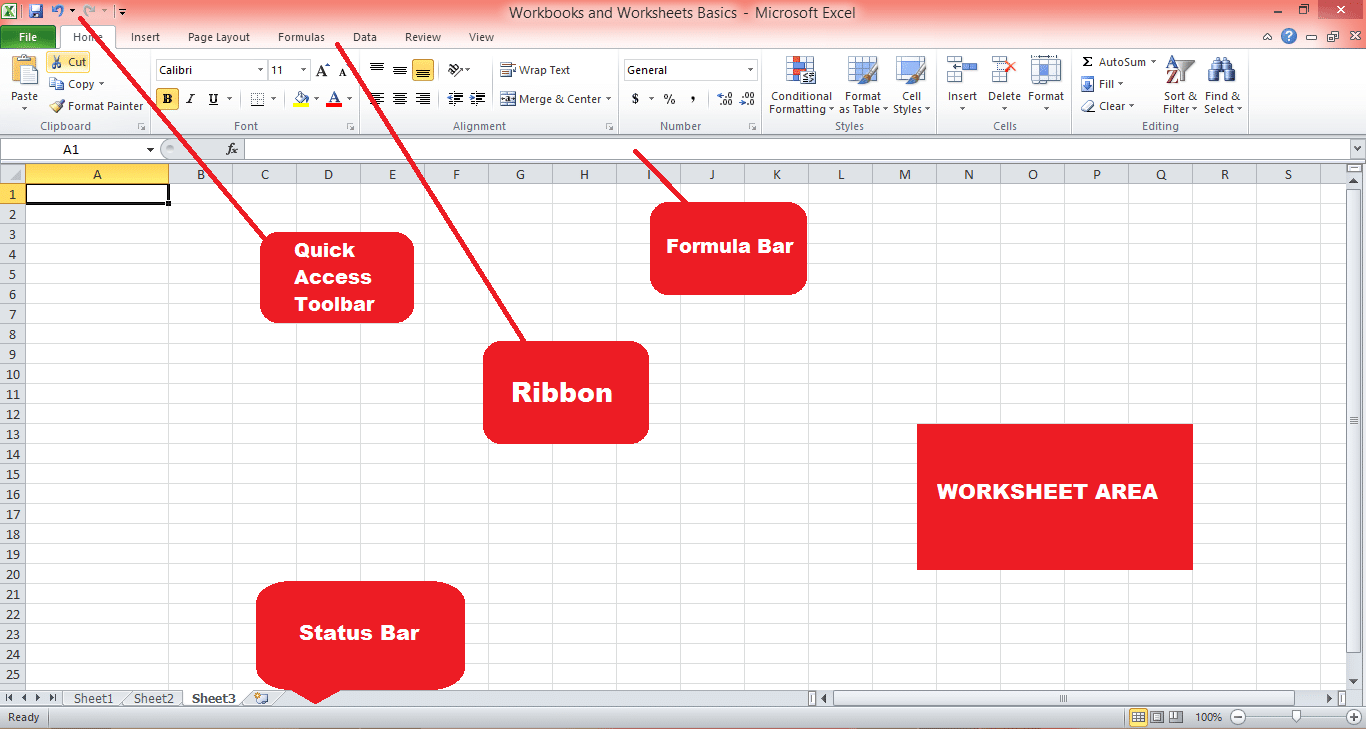
Microsoft Excel’s interface is designed to be user-friendly and intuitive. Key components of the interface include:

Ribbon: The Ribbon is a toolbar located at the top of the Excel window, containing various tabs (Home, Insert, Page Layout, etc.) that group related commands and features. You can customize the Ribbon by adding or removing tabs, groups, and commands.
Quick Access Toolbar: Located above the Ribbon, the Quick Access Toolbar provides shortcuts to frequently used commands, such as Save, Undo, and Redo. You can customize the Quick Access Toolbar by adding or removing commands.
Formula Bar: The Formula Bar, located below the Ribbon, displays the content of the active cell and allows you to edit formulas, text, calculate data, and more.
Worksheet Area: The Worksheet Area, the main working area in MS Excel, contains cells organized in rows and columns. Each cell can store data, such as text, numbers, or formulas.
Status Bar: Located at the bottom of the MS Excel window, the Status Bar provides information about the current worksheet, such as the number of selected cells, the average or sum of selected values, and the current mode (Ready, Edit, or Enter).
In the next section, we take a look at MS Excel workbooks and Excel spreadsheets and how you can effectively use them.
Understanding Workbooks and Worksheets
There are two fundamental building blocks of Excel: workbooks and worksheets.
A workbook is an Excel file that can store and organize multiple related worksheets. It has a file extension of .xlsx, .xls, or .xlsm, depending on the version of MS Excel and whether it contains macros. Workbooks allow you to keep related data together, making it easy to navigate, analyze, and maintain your information. You can think of a workbook as a binder that contains different sheets, each holding a separate set of data.
A worksheet, on the other hand, is an individual sheet or page within a workbook. Each worksheet is a grid of cells organized in rows (numbered) and columns (lettered), where you can enter, manipulate, and analyze data. By default, a new Excel workbook contains one worksheet, but you can add, remove, or rename worksheets as needed. Worksheets can be used to store different types of data, perform calculations, or create charts and visualizations.
Understanding how workbooks and worksheets function, as well as how to navigate and manage them efficiently, is essential for effectively organizing and working with your data.
This section will provide an overview of how to create and manage workbooks and worksheets, their features, and best practices for utilizing them in Microsoft Excel.
1. Creating and managing workbooks
To create a new Excel workbook, open up your version of the spreadsheet program and click “File” > “New” > “Blank workbook” or use the keyboard shortcut “Ctrl + N” (Windows) or “Cmd + N” (macOS).
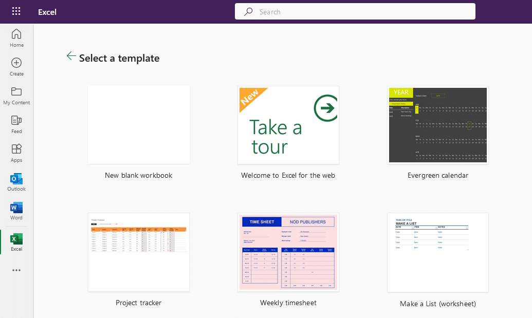
You can also create a workbook based on a template by selecting one from the available options. To open an existing workbook, click “File” > “Open” and browse to the location of your Excel files.
2. Adding, renaming, and deleting worksheets
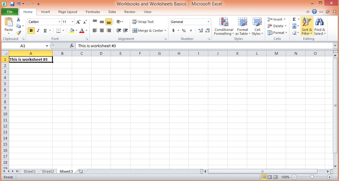
By default, a new workbook contains one worksheet. To add a new Excel worksheet, click the “+” icon next to the last worksheet tab, right-click an existing worksheet tab and select “Insert,” or use the keyboard shortcut “Shift + F11.”
To rename a worksheet, double-click the worksheet tab, type the new name, and press “Enter.” To delete a worksheet, right-click the worksheet tab and select “Delete.”
3. Navigating between worksheets
To move between worksheets, click the desired worksheet tab or use the keyboard shortcuts “Ctrl + Page Up” (previous worksheet) and “Ctrl + Page Down” (next worksheet) on Windows, or “Option + Left arrow” (previous worksheet) and “Option + Right arrow” (next worksheet) on macOS.
4. Grouping and ungrouping worksheets
Grouping worksheets allow you to perform actions on multiple worksheets simultaneously. To group worksheets, click the first worksheet tab, hold “Shift” or “Ctrl” (Windows) or “Shift” or “Cmd” (macOS), and click the other worksheet tabs you want to group. To ungroup worksheets, right-click any worksheet tab and select “Ungroup Sheets.”
In the next section, we take a look at how you can work with cells, columns, and rows in an Excel spreadsheet.
Working with Cells, Rows, and Columns
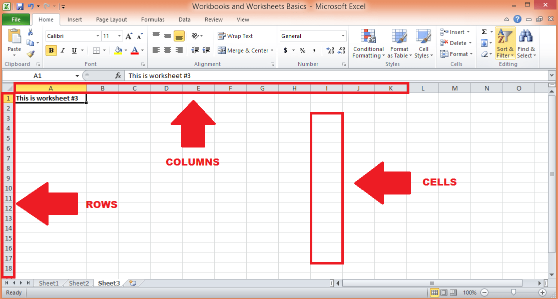
This section focuses on the core elements of Excel spreadsheets’ grid-like structure: cells, rows, and columns. Mastering the art of working with these components is crucial for managing and manipulating data within Excel files effectively.
We will discuss various techniques for selecting, editing, and formatting cells, rows, and columns, as well as tips for optimizing your workflow when working with these fundamental building blocks.
1. Selecting cells, rows, and columns
Click a cell to select it or click and drag to select multiple cells. To select an entire row or column, click the row number or column letter. To select multiple rows or columns, click and drag the row numbers or column letters. Use “Ctrl + A” (Windows) or “Cmd + A” (macOS) to select the entire worksheet.
2. Inserting and deleting rows and columns
To insert a row or column, right-click the row number or column letter and select “Insert.” To delete a row or column, right-click the row number or column letter and select “Delete.”
3. Adjusting row height and column width
To adjust row height or column width, click and drag the border of the row number or column letter. To autofit row height or column width based on the content, double-click the border. Check out this guide for more information.
4. Formatting cells
Formatting data in a Microsoft Excel spreadsheet is important because it helps to make your data more readable and understandable.
Spreadsheet cells can store different types of data, such as text, numbers, or dates, and MS Excel provides various formatting options to improve the appearance and readability of your data, such as:

Number formats: To change the number format (e.g., currency, percentage, date), select the cells and choose the desired format from the “Number” group on the “Home” tab.
Text alignment: To align text within cells, select the cells and choose the desired alignment option (left, center, right, top, middle, bottom) from the “Alignment” group on the “Home” tab.
Borders and shading: To apply borders or shading to cells, select the cells, click the “Border” or “Fill” button in the “Font” group on the “Home” tab, and choose the desired option.
5. Using cell styles and conditional formatting
Cell styles are predefined formatting options that can be applied to cells to visually organize and emphasize data. Conditional formatting allows you to apply formatting based on specific conditions, such as highlighting the highest or lowest values in a range. To apply cell styles or conditional formatting, select the cells, click the “Cell Styles” or “Conditional Formatting” button in the “Styles” group on the “Home” tab, and choose the desired option.
Now that you’re familiar with workbooks and worksheets and how to manage cells, rows, and columns, let’s take a look at some basic and a few advanced Microsoft Excel functions.
Let’s start with the basics.
What Are The Basic Microsoft Excel Functions?
Excel provides a wide range of built-in functions to perform calculations and manipulate data. Functions can be categorized into various types, such as arithmetic, text, date and time, and logical functions.
Let’s explore some of the most important ones.
1. Arithmetic operations
Excel offers basic arithmetic functions like SUM, AVERAGE, MIN, MAX, and COUNT, among others. To use a function, type “=” in a cell, followed by the function name and its arguments in parentheses. For example, “=SUM(A1:A10)” gives the sum of the contents in the range A1 to A10.
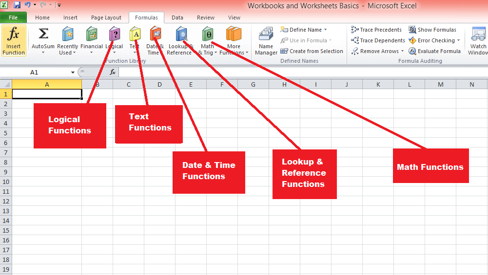
2. Text functions
Text functions, such as CONCATENATE, LEFT, RIGHT, MID, LEN, and TRIM, help manipulate and analyze text data. For example, “=CONCATENATE(A1, ” “, B1)” combines the text from cells A1 and B1 with a space in between.
3. Date and time functions
Date and time functions, such as TODAY, NOW, DATE, TIME, YEAR, MONTH, and DAY, allow you to work with date and time data. For example, “=DATEDIF(A1, TODAY(), “Y”)” calculates the number of years between the date in cell A1 and today.
4. Logical functions
Logical functions, such as IF, AND, OR, and NOT, enable decision-making based on specific conditions. For example, “=IF(A1>100, “High”, “Low”)” is an if function that returns “High” if the value in cell A1 is greater than 100 and “Low” otherwise.
5. Lookup and reference functions
Lookup and reference functions, such as VLOOKUP, HLOOKUP, INDEX, and MATCH, help you find and retrieve data from a table or range. For example, “=VLOOKUP(A1, B1:C10, 2, FALSE)” searches for the value in cell A1 within the first column of the range B1:C10 and returns the corresponding value from the second column.
The next section covers more advanced Excel functions, which have a learning curve and may need some practice to properly master, so yourself strap in!
What Are Some Advanced Microsoft Excel Functions?
As you progress in your Excel journey, harnessing the power of advanced Excel functions becomes essential for tackling complex data analysis and problem-solving tasks.
In this section, we will explore some of the most powerful and versatile advanced functions that Excel has to offer.
By understanding and applying these functions, you will elevate your data manipulation capabilities, streamline your workflow, and unlock new possibilities for extracting valuable insights from your data.
1. Statistical functions
Statistical functions, such as AVERAGEIF, STDEV, CORREL, and FORECAST, perform statistical analysis on data sets. For example, “=AVERAGEIF(A1:A10, “>100″)” calculates the average of the values in the range A1:A10 that are greater than 100.
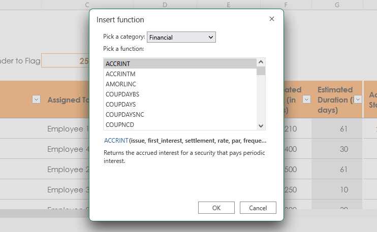
2. Financial functions
Financial functions, such as PMT, FV, NPV, and IRR, enable complex financial calculations, including loan payments, future value, net present value, and internal rate of return. For example, “=PMT(0.05/12, 360, -100000)” calculates the monthly payment for a 30-year loan of $100,000 with an annual interest rate of 5%.
3. Array formulas and functions
Array formulas and functions, such as TRANSPOSE, MMULT, and FREQUENCY, perform calculations on arrays of data. To create an array formula, type the formula in a cell, select the desired range, and press “Ctrl + Shift + Enter” (Windows) or “Cmd + Shift + Enter” (macOS).
4. Database functions
Database functions, such as DSUM, DAVERAGE, and DCOUNT, perform calculations on data stored in Excel tables or databases. For example, “=DSUM(A1:C10, “Amount”, E1:F2)” calculates the sum of the “Amount” column in the range A1:C10, based on the criteria specified in the range E1:F2.
Next, we take a look at how you can create and manage tables in Excel, which give a structured way to organize, analyze, and manipulate data. Tables offer several benefits, such as automatic formatting, easier data entry, and dynamic ranges.
How to Create and Manage Tables with Excel
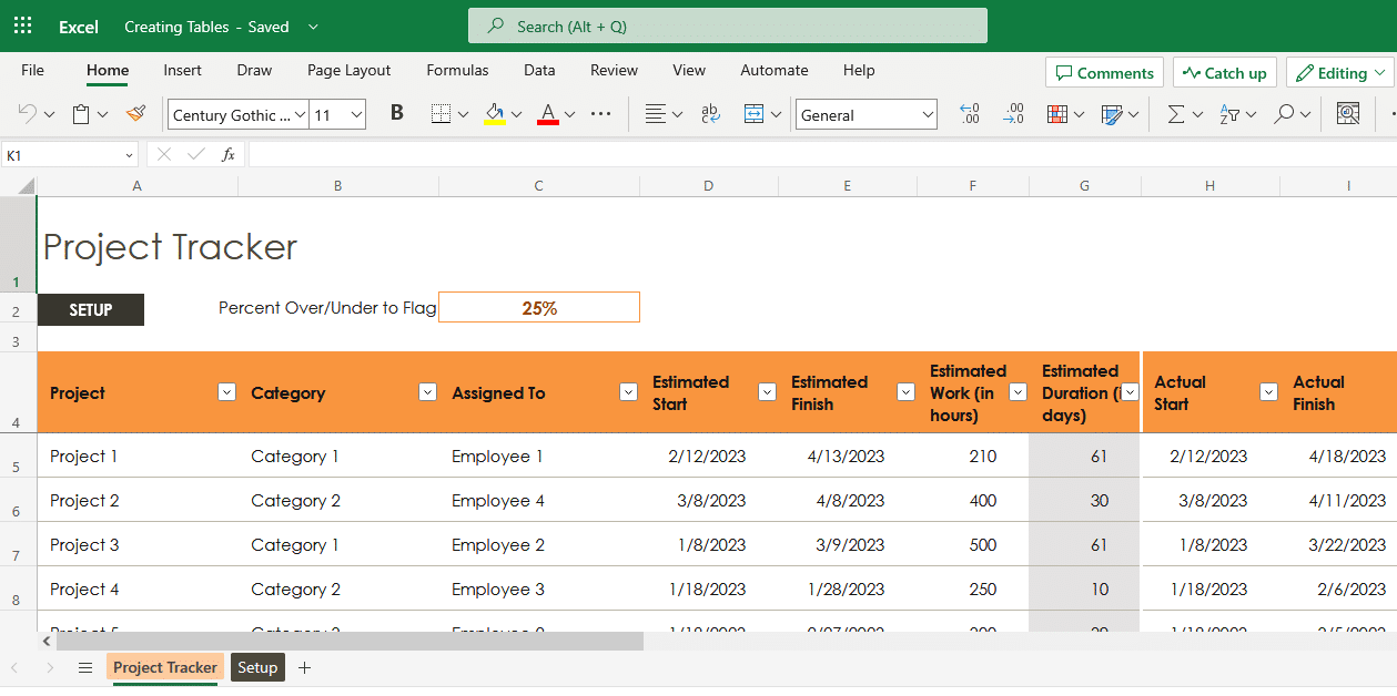
This section examines the process of creating and managing Excel tables, a powerful and flexible feature that simplifies data organization and analysis. Excel tables provide a structured format for your data, along with enhanced functionality for sorting, filtering, and formatting.
By learning how to create and effectively manage Excel tables, you can optimize your data handling and analysis, ensuring a more efficient and streamlined approach to working with your data sets.
1. Creating tables
To create a table, select the range of data, click “Table” in the “Tables” group on the “Insert” tab, and choose “New Table” or use the keyboard shortcut “Ctrl + T” (Windows) or “Cmd + T” (macOS).
2. Sorting and filtering data
Sorting and filtering data in a table can help you quickly find and analyze specific information. To sort data, click the drop-down arrow in the column header and choose the desired sort order (ascending or descending). To filter data, click the drop-down arrow in the column header, check or uncheck the values you want to display, and click “OK.”
3. Using slicers and timelines
Slicers and timelines provide a visual way to filter and arrange data together in a table. To insert a slicer, click the table, click “Slicer” in the “Sort & Filter” group on the “Table Design” tab, and choose the desired column. To insert a timeline, click the table, click “Timeline” in the “Sort & Filter” group on the “Table Design” tab, and choose the desired date column.
4. Data validation and data entry forms
Data validation helps ensure that data entered into a table meets specific criteria, such as a specific range of numbers or a list of allowed values. To apply data validation, select the cells, click “Data Validation” in the “Data Tools” group on the “Data” tab, and choose the desired validation criteria.
Data entry forms provide a user-friendly way to enter data into a table. To create a data entry form, click the table, click “Form” in the “Data Tools” group on the “Data” tab, and enter the data in the form.
5. Removing duplicates
To remove duplicate rows from a table, click the table, click “Remove Duplicates” in the “Data Tools” group on the “Table Design” tab, and choose the table array and columns to compare for duplicates.
What Are Excel Charts and Visualizations?
Let’s delve into the world of Excel charts and visualization, an essential aspect of effectively presenting and communicating data insights. Excel offers a wide range of chart types and visualization tools that enable you to transform raw data into meaningful and visually appealing representations.
By mastering the art of creating and customizing Excel charts, you can bring your data to life, making it easier to understand, analyze, and share with your audience.
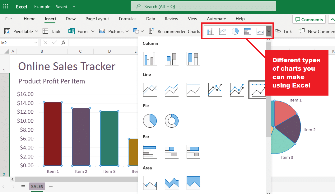
1. Types of charts
Excel offers numerous chart types to suit different data visualization needs, including:
Column and bar charts: Display data using vertical or horizontal bars, useful for comparing values across categories.
Line and area charts: Display data using lines or filled areas, useful for showing trends over time.
Pie and doughnut charts: Display data using segments of a circle, useful for showing the proportions of a whole.
Scatter and bubble charts: Display data using points or bubbles, useful for showing relationships between two or three variables.
Histograms and box plots: Display data using bars or boxes, useful for showing frequency distributions or statistical summaries.
2. Creating and modifying charts
To create a chart, select the data, click “Insert” > “Charts” and choose the desired chart type, or use the recommended charts feature for suggestions. To modify a chart, click the chart to display the “Chart Design” and “Format” tabs, which provide various options for customizing the chart’s appearance, layout, and data.
3. Using Sparklines
Sparklines are miniature charts that fit within a single cell, useful for showing trends or variations in data within a row. To create a sparkline, select the cell where you want to insert the sparkline, click “Insert” > “Sparklines,” choose the desired sparkline type (Line, Column, or Win/Loss), and specify the data range.
4. Conditional formatting with icon sets and data bars
Conditional formatting in Excel allows you to apply specific formatting, such as colors or icons, to cells based on their values or specific conditions. Icon sets and data bars are two types of conditional formatting that can help you visually represent data, making it easier to identify trends, patterns, or outliers.
a) Icon sets
Icon sets are a group of icons that can be applied to cells based on specified criteria. Excel provides various icon sets, such as arrows, traffic lights, and flags, to represent different data scenarios.
When you apply an icon set, Excel divides the data into three or more categories and assigns a specific icon to each category.
To apply an icon set:
Select the cells you want to format.
Click “Conditional Formatting” in the “Styles” group on the “Home” tab.
Choose “Icon Sets” and select the desired icon set from the list.
To customize the criteria for each icon, click “Conditional Formatting” > “Manage Rules” > “Edit Rule” and adjust the settings in the “Edit Formatting Rule” dialog box.
b) Data bars
Data bars are horizontal bars that represent the relative value of a cell within a range of cells. Data bars can help you quickly visualize the magnitude of values, making it easy to spot high and low values at a glance.
You can customize the appearance of data bars, such as the color, gradient, and border. To apply data bars:
Select the cells you want to format.
Click “Conditional Formatting” in the “Styles” group on the “Home” tab.
Choose “Data Bars” and select the desired color or gradient fill from the list.
To customize the appearance of data bars or modify the value range, click “Conditional Formatting” > “Manage Rules” > “Edit Rule” and adjust the settings in the “Edit Formatting Rule” dialog box.
By using conditional formatting with icon sets and data bars, you can enhance the visual appeal of your data and make it easier for your audience to understand and analyze the information.
Now, let’s talk about PivotTables and PivotCharts
What Are Excel PivotTables and PivotCharts?
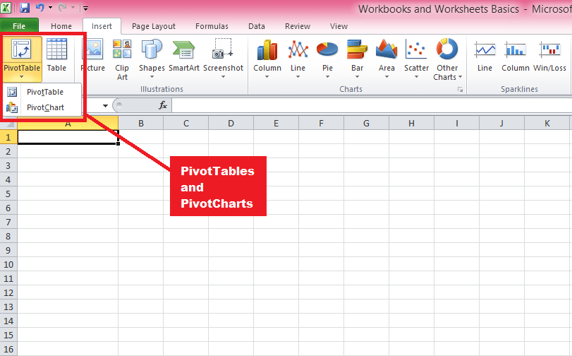
PivotTables and PivotCharts are powerful tools in Excel that enable you to summarize, analyze, and explore large data sets by organizing data in a hierarchical structure and presenting it in a visually appealing manner.
They allow you to manipulate data with simple drag-and-drop actions, making it easy to identify trends, patterns, and relationships within your data.
Let’s first discuss PivotTables
a) PivotTables
PivotTables are a powerful data analysis tool in Excel that allows you to summarize, organize, and explore large volumes of data in a structured, hierarchical format. They can be used to perform a wide range of tasks, such as data aggregation, cross-tabulation, and data filtering.
Below are the steps to follow to create them:
Creating PivotTables: Select the data you want to analyze, then click “Insert” > “PivotTable,” and choose the desired location for the PivotTable. Alternatively, you can use the “Recommended PivotTables” feature for suggestions based on your data.
Arranging and manipulating data in PivotTables: To organize your data, drag fields from the field list to the row, column, value, and filter areas. Change the summary function, apply number formatting, group data, and sort and filter data using various options available in the PivotTable context menus and the “PivotTable Analyze” tab.
Using calculated fields and items: You can perform custom calculations in PivotTables using formulas that reference other fields or items. Click “Formulas” > “Calculated Field” or “Calculated Item” in the “Tools” group on the “PivotTable Analyze” tab, and enter the formula in the “Formula” box.
Refreshing and updating PivotTables: You must refresh the PivotTable to update the summary calculations and display the latest data when the source data changes. Click “Refresh” in the “Data” group on the “PivotTable Analyze” tab or use the keyboard shortcut “Alt + F5” (Windows) or “Cmd + Option + R” (macOS).
b) PivotCharts
PivotCharts are dynamic, interactive charts based on PivotTables that enable you to visualize complex data relationships in a visually appealing manner.
They inherit the structure and data manipulation capabilities of PivotTables, allowing you to create, customize, and explore different data views by changing the layout, appearance, or summary calculations of the underlying PivotTable.
PivotCharts are an excellent tool for presenting and analyzing data in a more intuitive and engaging way. Below are the steps for creating PivotCharts
Creating PivotCharts: Click the PivotTable you want to create a chart for. b. Click “PivotChart” in the “Tools” group on the “PivotTable Analyze” tab, and choose the desired chart type.
Customizing and interacting with PivotCharts: Use the “Chart Design” and “Format” tabs to modify the chart’s appearance, layout, and data. Use the PivotTable field list, slicers, and timelines to interact with the chart and explore different data views.
By becoming proficient with PivotTables and PivotCharts, you can efficiently analyze and present complex data sets and uncover valuable insights. These tools are essential for anyone working with large amounts of data in Excel, especially when dealing with business, financial, or statistical analysis.
Next, we take a look at the importance of collaboration and sharing in Excel and learn how to effectively share your work with others, further enriching your Excel experience and optimizing your workflow.
How to Collaborate and Share Excel Files?
In today’s fast-paced and interconnected world, effective collaboration and sharing are crucial for successful teamwork and project management. Excel offers various features and tools that enable users to collaborate seamlessly and share their work with others.
This section will discuss some key aspects of collaboration and sharing in Excel, highlighting essential features and best practices.
1. Real-Time Collaboration
Excel supports real-time collaboration, allowing multiple users to work on the same spreadsheet or workbook simultaneously. This feature is available in Excel for Microsoft 365, Excel Online, and Excel mobile apps. To collaborate in real-time:
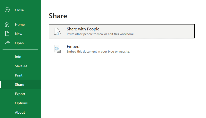
Save the workbook to a shared location, such as OneDrive or SharePoint.
Share the workbook with your collaborators by clicking “Share” in the upper-right corner of the Excel window and entering their email addresses or generating a sharing link.
Collaborators can open the shared workbook and make changes simultaneously, with changes being visible to all users in real-time.
2. Co-Authoring
Co-authoring is an integral part of real-time collaboration in Excel, allowing users to work on different parts of a workbook without overwriting each other’s changes. Excel automatically merges changes made by multiple users, while also providing options to review and resolve conflicts if they occur.
3. Version History
Excel keeps track of the version history for shared workbooks, enabling users to view, restore, or compare previous versions of a workbook. To access version history:
Click “File” > “Info” > “Version History” in Excel for Microsoft 365, or click the file name in the title bar and select “Version History” in Excel Online.
Browse through the list of previous versions, and click a version to open it in a separate window for review or comparison.
4. Comments and @Mentions
Excel provides a built-in commenting system that allows users to leave notes, ask questions, or provide feedback on specific cells or ranges. By using @mentions, you can tag collaborators in comments, notifying them and directing their attention to specific points in the workbook. To add a comment:
Select the cell or range you want to comment on.
Click “Review” > “New Comment” in Excel for Microsoft 365 or click “Insert” > “Comment” in Excel Online.
Type your comment and use @ followed by a collaborator’s name or email address to mention them.
Excel’s collaboration and sharing features make it easy for users to work together on projects, share insights, and streamline communication. By leveraging these tools and best practices, you can enhance your team’s productivity and ensure that your work is always up-to-date and accessible to those who need it.
In the next section, we take at look you can further expand Excel’s capabilities by using add-ins and its ability to integrate with various Microsoft products.
Excel Add-Ins and Integration with Other Microsoft Products
Excel’s capabilities can be significantly expanded through add-ins and integration with other Microsoft products, allowing users to perform advanced tasks, automate processes, and enhance their data analysis and visualization.
This section will discuss some of the most popular and useful Excel add-ins, as well as Excel’s integration with other Microsoft products, such as Power BI, Microsoft Word, and others.
What are Excel Add-ins?
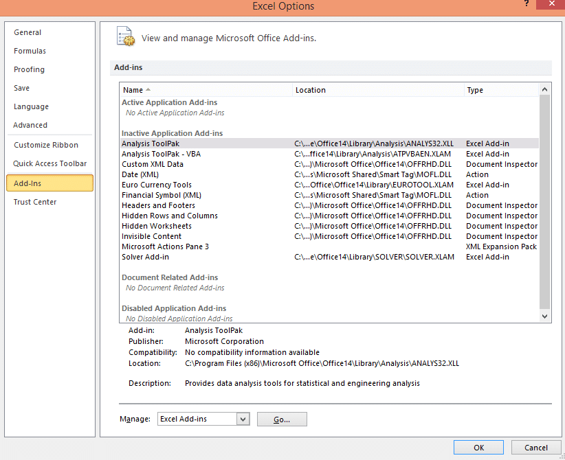
Add-ins are third-party extensions or plugins that can be installed within Excel to provide additional functionality. There are numerous add-ins available, ranging from data analysis tools to productivity enhancers.
Some popular Excel add-ins include:
Analysis ToolPak: A built-in Excel add-in that provides advanced statistical analysis tools, such as regression, correlation, and time series analysis.
Solver: A built-in optimization tool that helps users find the optimal solution for linear and nonlinear problems, including resource allocation, scheduling, and financial planning.
Power Query: A powerful data transformation and shaping tool that enables users to connect to various data sources, clean and transform data, and load it into Excel for further analysis.
Power Map: A 3D data visualization tool that allows users to create interactive geographic visualizations using geospatial data in Excel.
2. Integration with Microsoft Products
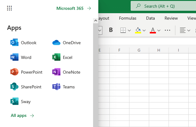
Excel seamlessly integrates with other Microsoft products, enabling users to leverage the strengths of multiple tools for a more comprehensive and efficient workflow. Some key integrations include:
Power BI: Power BI is a powerful data visualization and business intelligence tool that integrates with Excel to create interactive, real-time dashboards and reports. Users can connect Power BI to Excel data sources, import Excel data models, and even embed Excel objects like PivotTables and charts directly into Power BI reports.
Microsoft Word: Excel integrates with Microsoft Word, allowing you to share data between the two applications easily. This integration enables users to perform tasks such as inserting data, tables, or charts into a Word document, or using Word to create formatted reports based on Excel data.
SharePoint: Excel integrates with SharePoint, allowing users to store, share, and collaborate on Excel workbooks within a SharePoint environment. This integration facilitates version control, access management, and real-time co-authoring.
OneDrive: OneDrive enables users to store and sync Excel files in the cloud, making them accessible from any device and ensuring that changes are automatically saved and synced across all platforms.
Excel’s add-ins and integration with other Microsoft products significantly enhance its capabilities and help users perform more advanced tasks and create more sophisticated analyses.
By leveraging these add-ins and integrations, particularly the powerful data visualization tool Power BI, you can unlock the full potential of Excel and streamline your workflow across multiple Microsoft applications.
In the next section, we will explore various real-world applications of Microsoft Excel, demonstrating how the features and capabilities we’ve explored so far can be utilized to address practical challenges and scenarios.
What Are Real-World Applications of Microsoft Excel?
1. Business and Finance
Microsoft Excel plays a pivotal role in various business and finance sectors. It is commonly used for data analysis, record-keeping, budgeting, and financial reporting. Excel provides an intuitive graphical user interface with features like built-in formulas, functions, and data analysis tools that enable users to make informed decisions based on their data.
Companies of all sizes utilize the software program to perform cost-benefit analysis, financial analysis, track their income and expenses, and forecast future financial trends. With its robust capabilities, it has become an essential tool in the world of finance, allowing professionals to create financial models, organize data, and ensure accurate and efficient data analysis.
2. Education
Microsoft Excel is widely used in educational institutions for various purposes. Teachers often employ Excel to organize students’ grades, track attendance, and calculate averages or percentiles. Its features, such as graphing tools and pivot tables, enable educators to present data in a more visually appealing manner, making it easier for students to understand complex concepts.
Students benefit from learning how to utilize Microsoft Excel to perform calculations, analyze results, and develop problem-solving skills. The software is an invaluable resource when conducting research or presenting findings, making it a versatile tool for academic work.
3. Personal Productivity
Microsoft Excel extends its usefulness beyond business and educational settings, as individuals often rely on it for personal productivity purposes. Excel allows individuals to manage their personal finances, create budgets, and track expenses with ease. With Excel’s wide array of formulas, users can conduct their calculations and analyze their data effectively.
Furthermore, Microsoft Excel is used for event planning, such as organizing guest lists, tracking RSVPs, and creating seating charts. Individuals also utilize the software to analyze personal data, such as workout routines, meal planning, and project timelines. Its versatility makes Microsoft Excel a valuable tool to enhance personal productivity in various aspects of daily life.
The Bottom Line
Microsoft Excel has grown to become the most popular spreadsheet software in the world for good reason. It’s a versatile and powerful tool for working with data, performing calculations, and creating visualizations.
This comprehensive guide has covered the basics of Microsoft Excel, including the interface, data entry, formatting, basic and advanced functions, tables, charts, PivotTables, collaboration, and Excel add-ins and integrations.
By understanding and mastering these features, you can increase your efficiency, streamline your workflow, and unlock the full potential of Excel for data analysis and presentation.
As you continue to work with Excel, remember that there are many online resources, tutorials, and forums available to help you learn more advanced features and techniques.
The more you use Excel, the more proficient you will become in handling and analyzing data, making it an invaluable skill in today’s data-driven world.
To learn more about Excel and how to use it, check out the tutorial below:


