
You’ve scrolled through your rows in Excel, having to flip back and forth between essential data that’s more than a row apart.
Freezing your header row was a lifesaver, but life would be better if all your crucial info stayed visible on one screen, right?
You can freeze one or two rows in Excel, making your work process even more efficient. To do so, follow these steps:

1. Open your Excel file and find the row number of the row you want to freeze.
2. Right-click on the row number below which you want to freeze scrolls.
3. Select “Freeze Panes” and “Freeze Panes” from the drop-down menu again.
4. Now, the top two rows of your Excel spreadsheet will be frozen.
In this article, we’ll show you how to accomplish this, walk you through some important notes and best practices, and show you how to utilize its benefits in your daily work routine.
Let’s get into it.

How to Freeze the Top Row of a Spreadsheet

If you’ve scrolled down a spreadsheet in Excel, you’ve probably noticed that the first row, especially with headers, will disappear from view. Using the Freeze Panes tool helps keep these important rows or columns in view at all times.
To freeze the top row of your spreadsheet:
Open your Excel file and locate the row number of the row you’d like to freeze.
Move just below the row you’d like to freeze.
Now, click the “View” tab at the top of the Excel window.
Find the “Window” section; this could also be the place where the “Prompt,” “Arrange All,” and other commands are listed.
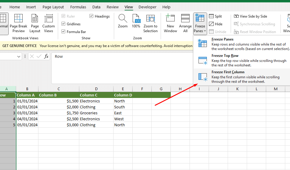
Click “Freeze Panes”. A drop-down menu with a few options will appear.
You can click on the “Qualifier” option and then click “Freeze Top Row,” or you can click “Split” to create a split view of your worksheet.
If you choose to split, you can click “Unfreeze panes” from the drop-down menu and select “Split” so that the row and the column will be frozen when you scroll down or to the right, respectively.
When you select the “Freeze Top Row” option, the top row of your spreadsheet will remain visible even if you scroll down, helping to keep your data organized and making your work more productive.
Let’s dive into how you can freeze not just one but two rows to keep crucial data always in sight
To freeze multiple rows in Excel, follow these steps:
Start by opening the Excel file where you want to freeze multiple rows.
For example, select the third row to freeze the first two rows. Click on the row number on the left side of the screen to select the entire row.
This tab is located at the top of the Excel window.
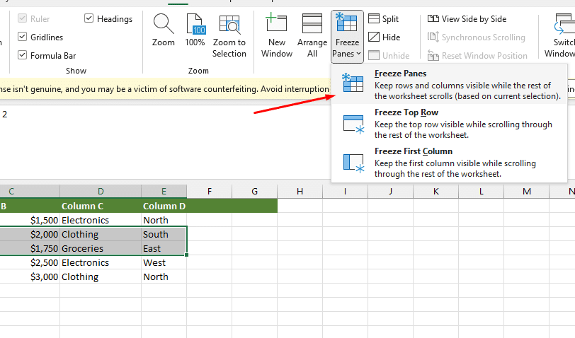
In the “Window” group of the “View” tab, you will find the “Freeze Panes” button.
A drop-down menu with a few options will appear.
The first option in the drop-down menu is usually “Freeze Panes.” Click on this option to freeze the rows above your selected row.
The rows above the selected row are now frozen. As you scroll down your spreadsheet, these rows will remain visible at the top of the screen.
How to Freeze the first column of your spreadsheet:
Locate the column letter you want to freeze.
Move just to the right of the column you’d like to freeze.
Click the “View” tab from the top of the Window.
Find the “Freeze Panes” button in the Window section.
Click “Top Row” or “First Column” from the drop-down menu, depending on your needs. The row or column you’ve selected will become fixed while the rest of the spreadsheet remains scrollable.
Besides freezing a single row, you can also freeze multiple rows in Excel.
This is handy, especially if you manage a larger dataset and want to keep several rows in view consistently.
Ready to enhance your Excel experience? Freezing panes instead of blocks can be a game-changer. Here’s the simple way to do it.
Why You Should Freeze Panes Instead of Blocks?
Working with large data sets in Excel often requires keeping specific rows or columns consistently visible, especially when scrolling through lengthy spreadsheets. This is where Excel’s Freeze Panes feature becomes invaluable.
Data Analysis Efficiency: When analyzing data, you often need to compare values across different spreadsheet sections. With Freeze Panes, your reference data, like headers or critical figures, stay visible, streamlining the comparison process.
Formula Tracking: If your spreadsheet involves complex calculations, Freeze Panes can help you keep track of your formula cells, making it easier to follow and verify your computations.
Multi-Sheet Comparison: Freeze Panes are not just limited to one sheet. When working with multiple sheets, you can freeze similar rows or columns in each sheet for a more coherent comparison.
Enhanced Readability: For large datasets, Freeze Panes improves readability by keeping vital information, like column headers, constantly in view.
In the next section, we’ll delve into some important considerations to remember when using the Freeze Panes feature in Excel.
Important Notes to Consider

Let’s take a look at some critical notes on how to maximize your Excel capabilities and avoid common pitfalls:
Impact on cursor position: When activating the first or top rows freeze, your cursor will go to the first or second cell at freezing positions. You’ll need to change the cursor location to your desired cell manually. The same goes for the first and top column freezes.
Freezing multiple rows and columns: You might need more than one row or column to be fixed on your Excel layout. Excel lets you achieve this by selecting the target cell to freeze the rows and columns above and to the left. You can only freeze the rows or columns on either side of the selected cell.
Freezing the top 2 rows in Excel: Use the Freeze Rows 1-2 option under the Freeze Panes menu. This technique can be helpful when working on extensive spreadsheets, researching, and comparing data.
Unfreezing panes: Sometimes, you may have locked panes that need to be freed. This can be done by selecting “Unfreeze Panes” from the ‘Freeze Panes’ drop-down in the ‘View’ tab.
Excel version compatibility: Ensuring that both users‘ Microsoft Excel versions support freeze pane features is critical when exchanging workbooks. This will help avoid inconsistencies in row/column visibility in shared documents.
Additional lock options: For more precise control over your spreadsheet and to ensure that essential rows and columns remain visible, you can use the “Split” option. It lets you create a static window within your sheet, which can be moved around as needed, allowing greater flexibility in keeping track of essential data.
We hope these helpful points will guide you to maintain an organized, user-friendly interface while working with your Excel spreadsheets.
Every now and then, you’re going to run into a problem! Let’s look at some of the common issues you may face.
Troubleshooting Common Issues When Freezing Rows

While it’s pretty straightforward to freeze rows, you might encounter situations where it’s not working as expected.
Understanding the underlying issues and their solutions will help you work more efficiently. Here are some common problems and their respective solutions:
1. No Freeze Pane option when clicking on headers
When you click on the headers, the selected row or cell is likely outside the visible area when the Freeze Pane option is unavailable in the drop-down menu.

To fix this, scroll to the top-left corner of your worksheet (cell A1).
2. Frozen rows are not visible
If the rows that should be frozen are not visible, it’s possible that you set up the freeze with an incorrect row selected.
In this case, go to View > Freeze Panes and select Unfreeze Panes to remove any existing freezes.
Then, ensure that you select the correct row or rows that you want to freeze before reapplying the freeze.
3. How to Unfreeze rows
When you want to unfreeze the rows you’ve frozen, click on Unfreeze Panes, and the rows will be free to move again.
Now, scroll up or down, and you’ll notice that the frozen rows will move along with the rest of the sheet.
Finally, Let’s reflect on some of our key takeaways.
Final Thoughts

Learning how to freeze rows in Excel gives you an edge when working with data. It makes navigation easier, lets you review header rows at all times, and keeps essential data visible even as you scroll.
Powerful and distinct, understanding this feature will make you swift and efficient as you immerse yourself in Excel’s data analysis capabilities.
Understanding how this method works will let you quickly and confidently navigate through scores of rows and columns, speeding up how you interact with your spreadsheets.
Do you want to learn more about interesting subjects like Power query? Checkout this great video on tracking changes using dimensions:
Frequently Asked Questions

What is the process to unfreeze the first 2 rows in Excel?
To unfreeze the first two rows in Excel, follow these steps:
Click on the View tab in your Excel ribbon.
Locate the Window group and click on the Freeze Panes button.
Select the Unfreeze Panes option from the drop-down menu.
This will unfreeze the rows, allowing you to scroll through the spreadsheet without the specified rows remaining fixed at the top.
How can I lock two rows on an Excel sheet?
You can lock two rows in Excel by freezing them. To do this, follow these steps:
Select the row right below the last row you want to freeze.
Go to the View tab in the ribbon.
In the Window group, click on Freeze Panes, and then select Freeze Panes.
This will lock the rows above the selected row and keep them visible as you scroll through the sheet.
Is it possible to freeze rows 1 and 2 in Excel?
To freeze both row 1 and row 2 in Excel, you’ll need to use the freeze panes feature.
First, select cell A3 of your worksheet.
Go to the View tab, then click on Freeze Panes.
Select the Freeze Panes option from the drop-down menu.
How do I set up the top 2 rows in Excel to freeze?
To freeze the top 2 rows in Excel, follow these steps:
Select the row beneath the last row you want to freeze. For example, if you want to freeze rows 1 and 2, select row 3.
Click on the View tab in the ribbon.
Find the Window group and click on the Freeze Panes button.
Select Freeze Top Row
What is best to pin names in the first and second rows?
Follow these steps to keep names visible as you scroll down in the first and second rows.
Select cell A3 in your Excel worksheet (below the names).
Go to the View tab and click on Freeze Panes.
In the drop-down menu, select ‘Freeze Panes‘.
This will freeze the first two rows in Excel, ensuring names are always visible at the top.


