
Locking formulas in Excel can help prevent accidental changes or deletions in your spreadsheet.
Are you ready to lock?
By doing this, you ensure that the calculated results remain accurate and consistent.

To lock formulas in Excel, you need to follow a few steps:
Select the cells where you want to apply the formula protection.
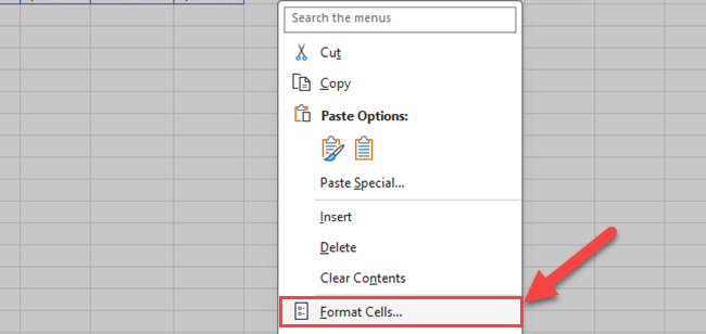
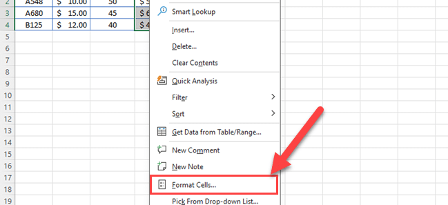
Right-click on the selected cells and choose “Format Cells”.
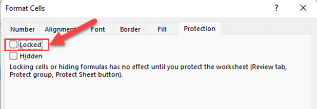
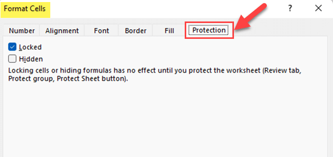
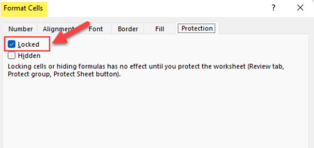
In the Format Cells window, go to the “Protection” tab and check the “Locked” checkbox.
Click “OK” to close the Format Cells window.
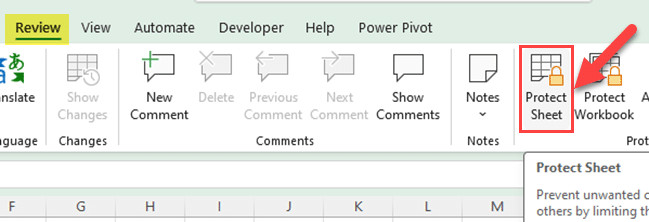
Go to the “Review” tab in the Excel ribbon and click “Protect Sheet.”
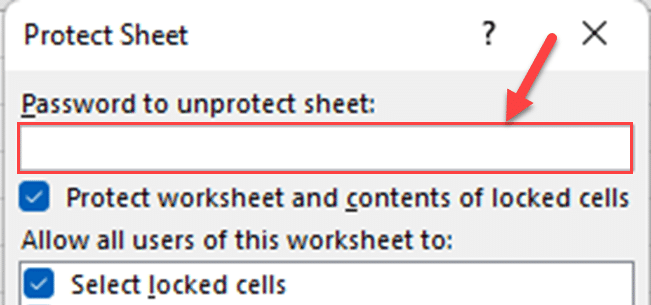
In the Protect Sheet window, enter a password (optional) and choose the specific actions you want to allow users to perform, such as selecting locked cells, formatting cells, or inserting/deleting rows and columns.
Click “OK” to protect the sheet.

After you have locked your formulas, you can be confident that your data will remain accurate and consistent.
Also, if you need to make changes to the locked cells, you can easily unprotect the sheet by following the same steps and entering the password (if you set one).
In this article, we’ll go over the process of locking Excel formulas in more detail, as well as discuss various protection options to help secure your spreadsheets.
Let’s get started!
How to Lock Formulas in Excel
Locking formulas in Excel is an important skill to have in your Excel toolbelt, one that can help maintain the integrity and security of your spreadsheet.

By locking cells containing formulas, you can prevent unwanted changes and ensure that the calculated results remain accurate.
To lock a formula, you’ll first need to protect the worksheet. Here are the steps to do so:
Step 1: Select All the Cells to Unlock
Right-click and select “Format Cells” from the context menu.
Uncheck the “Locked” checkbox and click “OK” to close the window.
Step 2: Select Cells to Lock
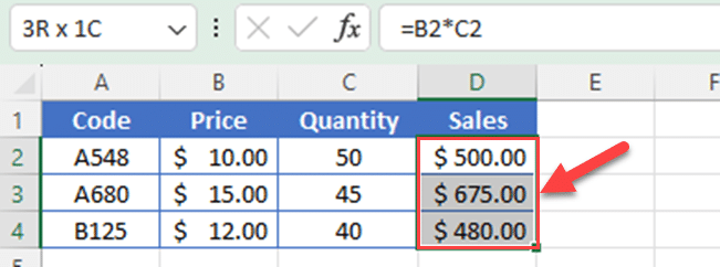
Select only the cells containing the formulas you want to lock.
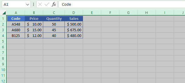
In the example below, we have selected the range D2:D4 which contains the formulas we want to lock.
Right-click on the selected cells and select “Format Cells” from the context menu.
Step 3: Protect the Worksheet
In the Format Cells window, go to the Protection tab.
Check the “Locked” checkbox and click “OK” to close the window.
Go to the Review tab in the Excel ribbon and click “Protect Sheet” in the Protect group.
Step 4: Finalize Protection Settings
In the Protect Sheet window, you can choose the specific actions you want to allow users to perform.
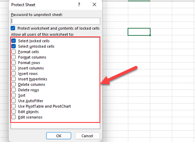
Enter a password (optional) and click “OK” to protect the sheet.
Your formulas are now locked, and your spreadsheet is protected from unwanted changes. Keep in mind that you’ll need to unprotect the sheet before making any adjustments to the locked cells.
To do this, follow the same steps. But, in the Review tab, you’ll see the unprotect sheet icon instead of the Protect Sheet icon.
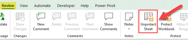
In the Unprotect Sheet window, enter the password you set (if any) and click “OK” to unprotect the sheet.
Additional Excel Formula Protection Techniques
In addition to the basic steps outlined above, Excel offers a variety of formula protection techniques to help safeguard your worksheets and ensure data integrity.
Let’s explore some of these advanced techniques below.
Hiding Formulas in Excel
In some cases, you may want to keep your formulas hidden while still displaying the results. Hiding formulas can be useful when sharing your spreadsheet with others or during presentations.
To hide a formula in Excel, you can use the following steps:
Step 1: Select the Cells with Formulas
Click and drag to select the cells or range of cells containing the formulas.
Step 2: Right-Click and Choose “Format Cells”:
Right-click on the selected cells, and choose “Format Cells” from the context menu.
Step 3: Go to the “Protection” Tab:

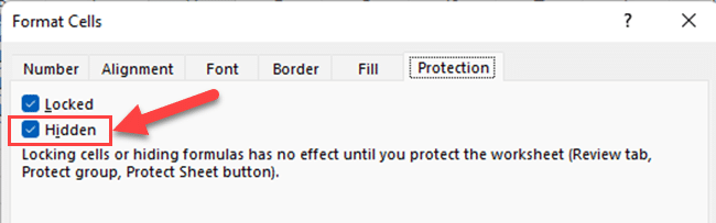
In the Format Cells dialog box, go to the “Protection” tab.
Step 4: Check the “Hidden” Option:
Check the “Hidden” option under the Protection tab.
Step 5: Click “OK”:
Click the “OK” button to apply the changes.
Step 6: Protect the Worksheet:
To actually hide the formulas, you need to protect the worksheet.
To do that, go to the “Review” tab and click on “Protect Sheet.” Set a password if needed and click “OK.”
Now, the formulas are visually hidden. To view them again, you need to unprotect the sheet.
Final Thoughts
By following the simple steps outlined in this article, you can confidently safeguard your critical calculations and share your work with peace of mind.
Whether you’re a seasoned Excel user or just starting, mastering formula protection will streamline your workflow and minimize errors.
So, go ahead and apply these techniques to your worksheets today. You’ll be one step closer to creating robust, professional-looking spreadsheets.
Want to learn more about Excel?
Do you want to become a pro at cleaning your data in your spreadsheet? Check out our video below!
Frequently Asked Questions
How can I protect a specific cell in Excel?
First, select the cell you want to protect, then right-click and choose “Format Cells.” In the “Format Cells” dialog box, go to the “Protection” tab and check the “Locked” checkbox.
Click “OK” to close the dialog box. After that, you can protect the entire sheet using the “Protect Sheet” option under the “Review” tab in the Excel ribbon. Now, the specific cell will be locked, and its contents cannot be changed unless the worksheet is unprotected.
What is the difference between locking cells and protecting a sheet in Excel?
Locking cells in Excel allows you to prevent specific cells from being edited, while protecting a worksheet enables you to restrict various actions, including editing, formatting, and sorting, on the entire worksheet.
When you lock a cell, you’re only preventing direct changes to its content, but protecting a sheet applies a broader range of restrictions.
Can I protect formulas from being changed in Excel?
Yes, you can protect formulas from being changed in Excel by locking the cells that contain the formulas. To do this, select the cells with the formulas, right-click, choose “Format Cells,” and go to the “Protection” tab.
Check the “Locked” checkbox and click “OK.” After that, protect the entire sheet using the “Protect Sheet” option under the “Review” tab in the Excel ribbon.

This will prevent any changes to the locked cells, including the formulas they contain.
How do I unlock a cell in Excel with a password?
To unlock a cell in Excel with a password, you’ll first need to unprotect the sheet. Go to the “Review” tab, click “Unprotect Sheet,” and enter the password if one was set during protection.
Then, right-click on the cell you want to unlock, choose “Format Cells,” go to the “Protection” tab, and uncheck the “Locked” checkbox. Click “OK,” and the cell will now be unlocked and editable. Don’t forget to protect the sheet again after making the necessary changes.


