How to Create P Value in Excel? A Step-by-Step Guide

Ready to create a P value in Excel? Want to learn how to quickly and efficiently do it? Read on.

To calculate p-values in Excel, you generally use the T-test statistical function for hypothesis testing. You can also use it to interpret the results of hypothesis tests and make informed decisions about your data.

In this article, you’ll learn what a p-value is, its importance, and how to calculate it using various techniques in Excel, such as the T.test function and ANOVA.

By the end, you’ll be equipped with the necessary knowledge and practical skills to expertly interpret p-values in Excel, improving your ability to draw meaningful conclusions from your data.

Let’s get Started!

What is a P-Value

A p-value provides a measure of the evidence against a null hypothesis. To understand this concept, let’s break down the different components.

• Hypothesis testing: In statistics, researchers test whether their results are due to true treatment effects or mere chance. This process involves formulating a null hypothesis ($H_0$) and an alternative hypothesis ($H_1$).
• Null hypothesis ($H_0$): This statement asserts no significant population parameter or distribution difference. If you are trying to determine if there’s an effect from a treatment, the null hypothesis might state that the treatment has no effect.
• Alternative hypothesis ($H_1$): This is the opposite of the null hypothesis. It states that there is a significant difference or effect.
• P-value: This is the probability of observing your data or something more extreme if the null hypothesis is true.

In hypothesis testing, you typically set a significance level, usually denoted as alpha ($\alpha$), a threshold for the p-value. If the p-value is less than or equal to the significance level, you reject the null hypothesis in favor of the alternative hypothesis.

On the other hand, if the p-value is more significant than the significance level, you fail to reject the null hypothesis. In other words, a low p-value indicates strong evidence against the null hypothesis, while a high p-value fails to provide strong evidence against it.

Now, let’s delve into how to effectively calculate p-values using Excel’s various functions and methods.

How to Calculate P-Values in Excel

There are various functions and methods in Excel that will help you calculate p-values. These include the T.subtract, T.dist, T.test, ChiSq.test, and ANOVA.

What are T-Test in Excel

T-tests are a family of statistical tests used to infer the population mean of a certain characteristic from a sample. There are three main types of t-tests in Excel:

• One-sample t-test: Compares the mean of a sample to a known value or hypothesized mean of the population.
• Independent (or unpaired) t-test: Compares the means of two unrelated (independent) groups.
• Paired t-test: Compares the means of two related (paired) groups.

The T.TEST function is a built-in Excel statistical function that calculates the p-value for a given sample.

It is used for two-tailed hypothesis testing and returns the probability associated with a t-value from a t-distribution.

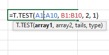
This function has the following syntax:

• T.TEST(known\_data, x, tails, type): Returns the two-tailed t-distribution probability given a sample and a constant.
• known\_data: The array or range containing the sample data.
• x: The value corresponding to the sample mean to be tested against the population mean.
• tails: A numerical value indicating the number of tails for the distribution (1 for one-tailed test, 2 for two-tailed test).
• type: An optional argument that specifies the type of t-test to be performed (1 for paired, 2 for two-sample with equal variance, and 3 for two-sample with unequal variance).

Next, we explore the process of conducting a t-test in Excel, a crucial step in hypothesis testing.

How to perform a t-test in Excel

1. Arrange your sample data in the Excel worksheet.
2. Use the T.TEST function to calculate the p-value for the respective t-test (one-sample, independent, or paired).

You can follow the sample syntax specific to each type of t-test as per your requirements.

• One-sample t-test syntax: =T.TEST(known\_data, x, 2, 1) for a one-tailed test or =T.TEST(known\_data, x, 2, 2) for a two-tailed test.
• Independent t-test syntax: =T.TEST(array\_1, array\_2, 2, 3).
• Paired t-test syntax: =T.TEST(array\_1, array\_2, 2, 1).

Let’s break down how to perform a one-sample t-test in Excel, a fundamental technique in statistical analysis.

How to perform a One-sample t-test

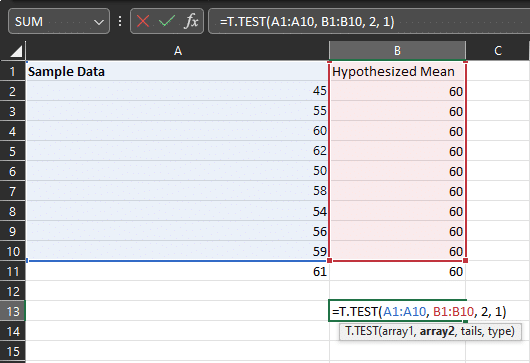
For example, if your sample data is in the range A1:A10, and you want to perform a one-sample t-test with a hypothesized mean of 60, with two tails, the formula would be =T.TEST(A1:A10, 60, 2, 2).

The result of this function will be the p-value, which indicates the likelihood of observing the sample mean given that the true population mean is equal to the specified value, using the specified tails and type of t-test.

By effectively understanding and using the T.TEST function, you can confidently perform t-tests and interpret their results in Excel.

Moving on, we examine the steps to conduct an ANOVA test in Excel, an essential tool for comparing multiple groups.

How to Perform an ANOVA Test in Excel

ANOVA (Analysis of Variance) is a statistical method used to evaluate whether there are statistically significant differences between the means of three or more independent groups.

In Excel, you can use the ANOVA: Single Factor Data Analysis Toolpak or the ANOVA function for Single Factor ANOVA.

Let’s look at these approaches in more detail.

1. ANOVA: Single Factor Data Analysis Toolpak

To perform a single factor ANOVA in Excel using the built-in tool, you first need to enable the Data Analysis ToolPak.

Here’s how to do it:

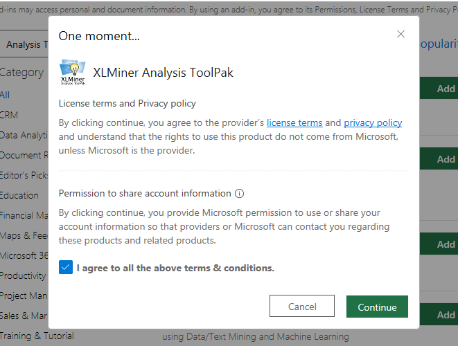
Get the XLMiner Analysis Toolpack

1. Click on the File tab, and then select Options.
2. In the Excel Options dialog box, click on Add-Ins.
3. In the Add-Ins dialog box, select Excel Add-Ins in the Manage box, and then click Go.
4. In the Add-Ins dialog box, check the Analysis ToolPak box, and then click OK.

Now that you have enabled the Data Analysis ToolPak, you can use it to perform a single-factor ANOVA as follows:

Perform a single-factor ANOVA

1. Click on the Data tab, and then click on Data Analysis.
2. In the Data Analysis dialog box, select ANOVA: Single Factor, and click OK.
3. In the Input Range box, enter the range of the data you want to analyze.
4. In the Grouping Information box, enter the range of the cell that contains the group labels for the data you want to analyze.
5. Select the appropriate Output Options, and click OK.

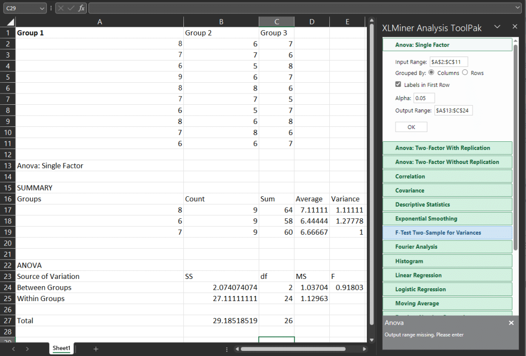
The result of this function is an ANOVA table, which includes the p-value associated with the F-statistic.

If the p-value is less than the significance level (usually set at 0.05), you can conclude that there is a significant difference between the means of at least two groups.

The ANOVA table also includes other information, such as the sum of squares, degrees of freedom, F-statistic, and within-group and between-group variances.

You can use this information to gain insights into the relationships between the data points and make informed decisions based on the statistical significance of the differences among the group means.

With Excel’s built-in ANOVA tool, you can confidently analyze your data and draw meaningful conclusions from your results.

Diving deeper, we’ll learn about the Chi-Square test in Excel and how it’s used to assess relationships between categorical variables.

Learning Chi-Square Test in Excel

The chi-square test is a statistical test that is used to determine whether there is a significant association between two categorical variables.

It is commonly used in fields such as science, medicine, and social sciences to analyze data and make inferences about the population.

The chi-square test is often used to test whether two categorical variables are independent of each other.

If the variables are independent, there is no relationship between them, while if they are dependent, there is a relationship between them.

In Microsoft Excel, you can easily perform a chi-square test on your data using the CHITEST function. This function, also known as the Pearson’s chi-square test, can be used to determine the p-value associated with the chi-square statistic.

Here’s an Example of a Chitest

=CHITEST(actual\_data, expected\_data)

The CHITEST function in Excel has the following syntax:

• actual\_data: This is the range of cells containing the observed frequencies or counts. These are the actual data you have collected.
• expected\_data: This is the range of cells containing the expected frequencies or counts. These are the values you expect to see if the null hypothesis is true.

The function will return the p-value associated with the chi-square test. You can then use this p-value to assess the significance of the relationship between the two categorical variables.

Now, let’s focus on how to apply the CHITEST function in Excel for a practical chi-square test.

How to use the CHITEST function

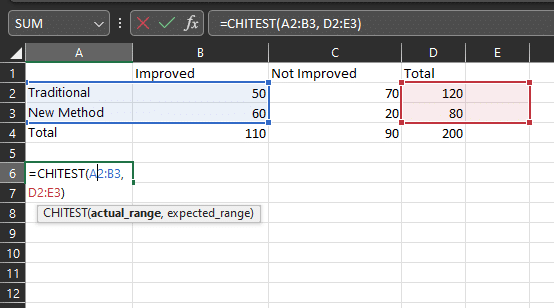
1. Organize your data. Create a table in Excel that displays the observed and expected frequencies for each category of the two categorical variables you are investigating.
2. Use the CHITEST function in a cell in your worksheet.
3. Press Enter. The result should be a p-value.

The chi-square test is useful for examining the relationship between two categorical variables. You can easily perform this test in Excel using the CHITEST function or the Data Analysis ToolPak.

The p-value from the test can help you make inferences regarding the significance of the relationship between the variables in your data.

The following sections will guide you on using the Excel statistical functions for t-tests, ANOVA, and chi-square tests to calculate p-values.

Next, we explore the various Excel statistical functions that are instrumental in calculating p-values.

Using Excel Statistical Functions

Excel provides a range of statistical functions to help you calculate p-values for your data. Some of the most commonly used Excel statistical functions are explained below.

1. T.SUBTRACT

The T.SUBTRACT function (also known as the “T.INV.2T” function) calculates the critical value from a t-distribution for a given significance level and degrees of freedom.

The formula for the T.SUBTRACT function is:

• =T.SUBTRACT(alpha, df)
• alpha: The significance level at which you conduct the hypothesis test (e.g., 0.05 for a 5% significance level).
• df: The degrees of freedom of the t-distribution (usually equal to the sample size minus 1 for a one-sample t-test).

T.INV.2T can help you calculate the p-value for t-tests, allowing you to determine the statistical significance of your findings.

2. T.DIST.2T

The T.DIST.2T function calculates the probability density function for two-tailed t-tests.

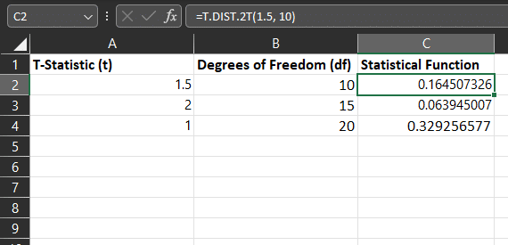
The syntax for the T.DIST.2T function is:

• =T.DIST.2T(t, df)
• t: The t-statistic for which you want to calculate the p-value.
• df: The degrees of freedom of the t-distribution.

The result of the T.DIST.2T function is a p-value, which represents the probability of observing a t-statistic as extreme as the one in the sample data, assuming the null hypothesis is true.

3. T.DIST

The T.DIST function calculates the probability density function for a given t-statistic and a set of degrees of freedom.

The t-distribution looks normal but differs depending on the sample size used for the t-test.

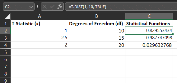
The syntax for the T.DIST function is:

• =T.DIST(x, df)
• x: The t-statistic for which you want to calculate the p-value.
• df: The degrees of freedom of the t-distribution.

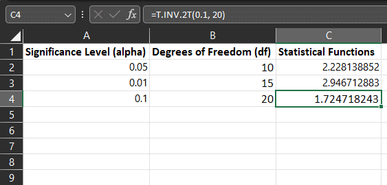
4. T.INV.2T

The T.INV.2T function (also known as the “T.INV” function) calculates the inverse of the two-tailed t-distribution.

This function can be helpful when you have the desired alpha level and must calculate the corresponding critical t-value.

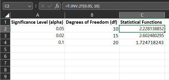
The syntax for the T.INV.2T function is:

• =T.INV.2T(alpha, df)
• alpha: The desired significance level (e.g., 0.05 for a 5% significance level).
• df: The degrees of freedom of the t-distribution.

5. T.TEST

The T.TEST function in Excel is used to perform a two-sample t-test.

The t-test is a statistical test used to determine whether a significant difference exists between the means of two independent groups.

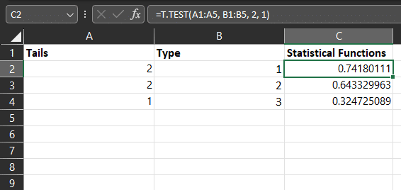
The syntax for the T.TEST function is:

=T.TEST(array1, array2, tails, type)

• array1: The first set of data.
• array2: The second set of data.
• tails: The type of test to perform: 1 for a one-tailed test, 2 for a two-tailed test.
• type: The type of t-test to perform: 1 for a paired test, 2 for a two-sample equal variance test, 3 for a two-sample unequal variance test.

If the T.TEST is two-tailed, the result of the function is the p-value.

If you have a one-tailed test, you need to divide it by 2.

If the test is greater or less than, you’ll have to use the following formulas: B1/2, B/(cell), and (1-B)/2. Remember to use the absolute value of the t-statistic for a less-than test.

The T.TEST function can also be used to interpret the results of a t-test.

The Excel statistical functions for calculating p-values are essential for hypothesis testing and inferential statistics. By utilizing these functions, you can confidently make decisions based on the probability of observing specific values in your data.

Mastering the calculation of p-values in Excel is vital for making informed decisions based on statistical analysis.

Final Thoughts

Calculating p-values in Excel is a crucial part of statistical hypothesis testing, enabling you to make informed decisions and draw meaningful conclusions.

The statistical functions available in Excel and the statistical analysis tools allow you to carry out a variety of hypothesis tests and calculate p-values with ease.

Understanding how to confidently perform T-tests, ANOVA, and Chi-Square tests to assess the statistical significance of your data sets is a valuable skill.

Mastering p-value calculations in Excel will help you make informed decisions based on your statistical analysis, ensuring the accuracy and reliability of your results.

So go on, give it a test, and see how easy it is to create a p value in Excel.

Do you want to learn how to supercharge you PowerBi development with chaGPT? Checkout the EnterpriseDNA Youtube Channel.

Frequently Asked Questions

What is a P-value in Excel?

A p-value in Excel is a statistical measure that helps you determine the significance of your findings in hypothesis testing. d

It represents the probability of obtaining a result at least as extreme as the one observed under the assumption that the null hypothesis is true.

Why is the P-value important in Statistical Analysis?

P-values are crucial in determining whether to reject or accept the null hypothesis. A low p-value (< 0.05, typically) suggests strong evidence against the null hypothesis, indicating that your findings are statistically significant.

How Can I Calculate a P-Value in Excel?

You can calculate p-values in Excel using various functions and tests, including T.TEST for t-tests, ANOVA for analysis of variance, and CHITEST for the chi-square test.

These functions compute the p-value based on your data and the statistical test you perform.

What are T-Tests, and How are They Used in Excel?

T-tests in Excel are used to compare sample means against a known population mean (one-sample t-test) or between two groups (independent or paired t-tests). Excel’s T.TEST function helps calculate the p-value for these tests.

What is ANOVA, and How is it Performed in Excel?

ANOVA (Analysis of Variance) is a method used to compare means between three or more groups. In Excel, you can perform ANOVA using the Data Analysis Toolpak or the ANOVA function.

It generates a table with the p-value, helping you assess the statistical significance of the differences among group means.

How Do I Use the Chi-Square Test in Excel?

The chi-square test in Excel, performed using the CHITEST function, assesses the association between two categorical variables.

It calculates the p-value, determining whether the observed association is statistically significant.

Are There Specific Excel Functions for Calculating P-Values?

Yes, Excel offers specific functions like T.SUBTRACT, T.DIST.2T, T.DIST, and T.INV.2T, each serving different purposes in the calculation of p-values, depending on the hypothesis test being conducted.

How Do I Interpret P-Values in Excel?

P-value interpretation depends on your set significance level (?). If the p-value is less than ? (usually 0.05), it suggests strong evidence against the null hypothesis. If it’s greater, it indicates insufficient evidence to reject the null hypothesis.

Can Excel Handle Different Types of T-Tests?

Yes, Excel can handle different types of t-tests, including one-sample, independent, and paired t-tests. The function syntax varies slightly depending on the test type.

Is It Possible to Perform Hypothesis Testing for Large Data Sets in Excel?

Yes, Excel is capable of handling large data sets for hypothesis testing. However, the process might be slow for extremely large data sets, and care must be taken to ensure accurate data entry and formula application.