How Can I Learn Excel Quickly: A How-To Visual Guide

Need to learn Excel quickly? You’ve come to the right place!

In this quick guide, we will get you up to speed with the basics so you know what to do and how to do it!

To learn Excel quickly, it’s important to familiarize yourself with its interface and get comfortable navigating through its various features. You should also take advantage of the extensive tutorials and training courses available online for both beginners and advanced users.

In this article, we’ll get you started with the basics and work from there.

So, let’s get started!

Getting Started with Excel Basics

Before we can start creating beautiful charts and analyzing our data in Excel, we first need to learn about its fundamentals. In this section, we’ll go over the basics of Excel:

How to Create Your First Excel Spreadsheet

Here’s how you can create your first spreadsheet in Excel:

• Open Excel and choose the blank workbook option.
• The new workbook will have a single sheet called Sheet1. Click on the Ctrl + S button to save it.
• In the Save As menu, select the Browse button. A window will open in your file system.
• Select where you want to save the workbook on your PC, specify a name for it, and click on save.

How to Explore the Excel Workspace

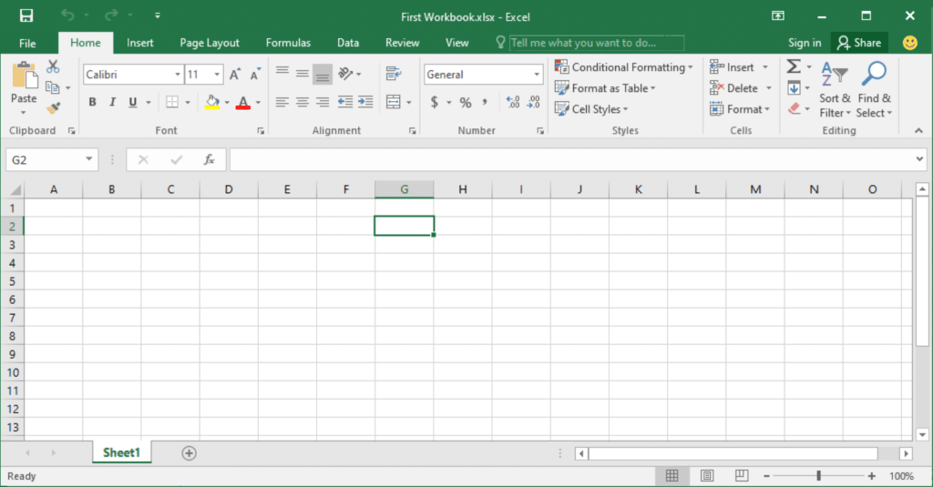
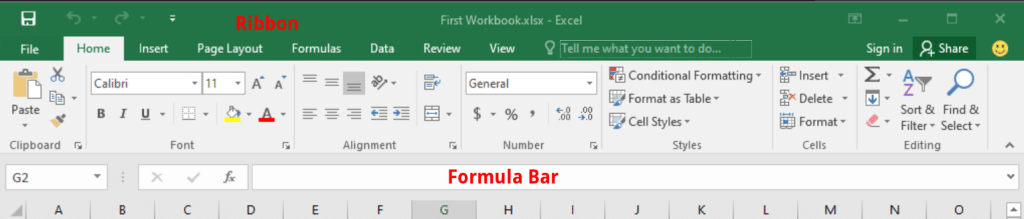
Congrats, you’ve created your first Excel Workbook! Now let’s explore it a bit. At the top, you’ll find the Ribbon, which hosts various tools and features organized into different tabs, like ‘Home’, ‘Insert’, ‘Formulas’, and ‘Data’.

Each tab contains relevant functions. For example, the ‘Home’ tab has options for formatting cells, text, and numbers, while the ‘Insert’ tab allows adding charts, tables, and graphics. Just below the ribbon, you’ll find the formula bar which provides a space for you to enter or edit Excel data and formulas into the current highlighted cell.

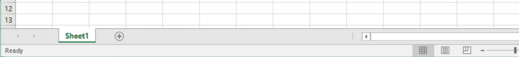
At the bottom of the spreadsheet, you’ll find the tabs for each sheet. Keep in mind that a workbook can contain multiple spreadsheets. You can add a new sheet to an Excel Workbook by clicking the plus icon at the bottom of the workbook.

Working with Cells, Rows, and Columns

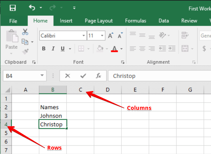
In the Excel workbook, the workspace comprises cells organized into rows and columns, with rows identified by numbers and columns with letters. A cell’s address combines its row and column, like A1 or B2.

Click on a cell to select it and begin entering data. Press Enter to move down a row or Tab to move to the next cell to the right. You can select entire rows or columns by clicking on the row number or column letter, respectively.

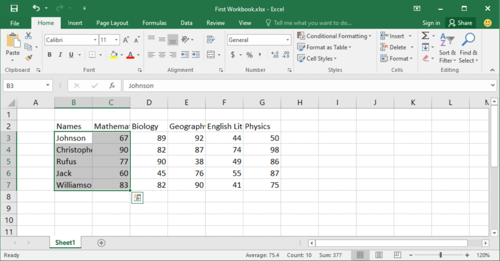
Let’s look at a real-world example of the test scores of some students in a school. Let’s enter their names and scores into our workbook.

You can select multiple cells by using the shift button plus the arrow keys. You can also specify the entire range of cells using the colon character. For example, if I want to specify the cells from B3 to C7 in a function, I can use the notation (B3:C7).

To insert or delete rows or columns, right-click on them and choose the appropriate option from the context menu.

How to Work with Formulas and Functions in Excel

We’ve now covered the basics of opening a workbook and filling it with data. Now, let’s look at how we can perform calculations on this data.

Performing Basic Calculations in Excel

In Excel, formulas allow you to perform calculations on your data. They can help you analyze, manipulate, and visualize data more effectively. To create a formula, simply enter an equal sign (=) in a cell, followed by an expression.

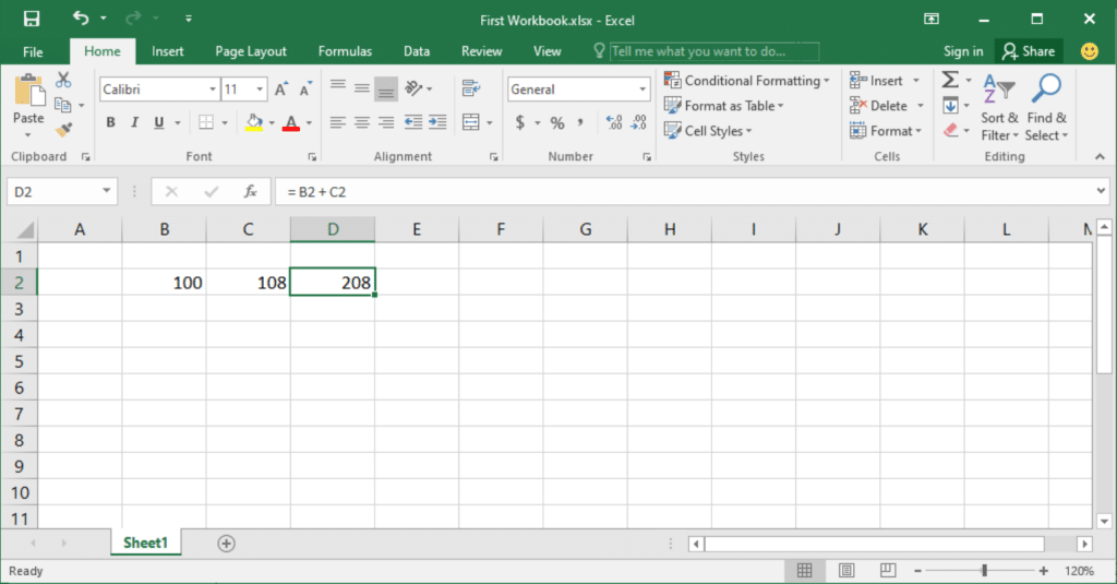
For example, to multiply 12 by 9 in cell C2, you can type = 12*9 in the cell. You can also perform calculations between two cells. For example, to add the values in cells B2 and C2, you can type =A2+B2 in D2.

Likewise, you can subtract, multiply, or divide by changing the operators to –, *, or /.

Mastering Common Functions

Excel also provides various built-in functions, which are powerful tools that help you perform more complex calculations and operations. Let’s look at some of the most common and widely used functions in Excel.

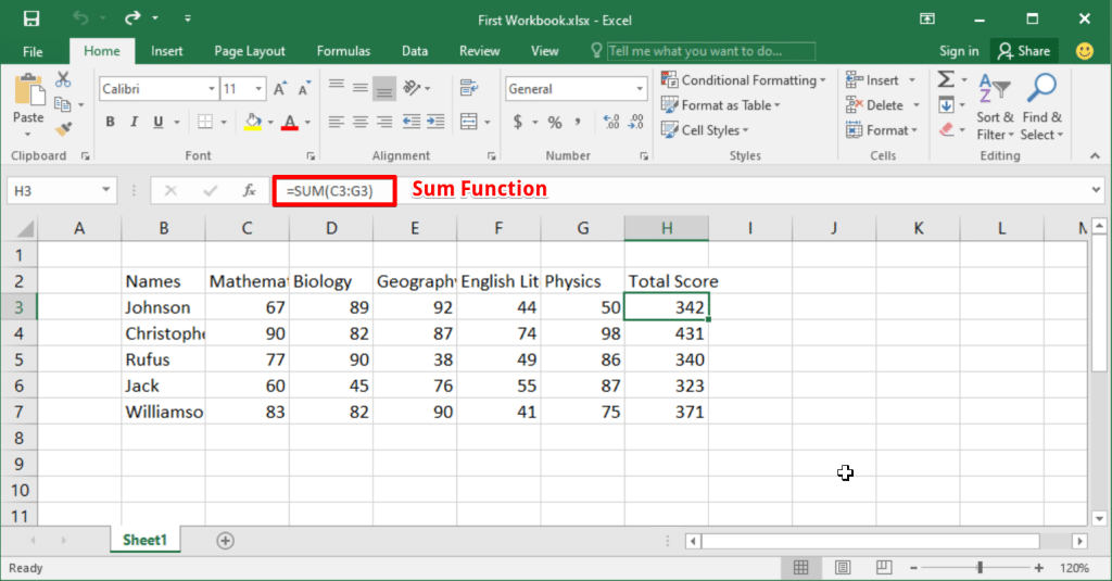
• SUM: To add a range of cells, you can use the SUM function. For example, =SUM(A1:A10) adds the values in cells A1 through A10. Let’s look at an example in our workbook by adding a Total score column for each student.

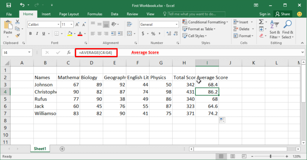
AVERAGE: Returns the average of the values in a specific range. Let’s add an average score column.

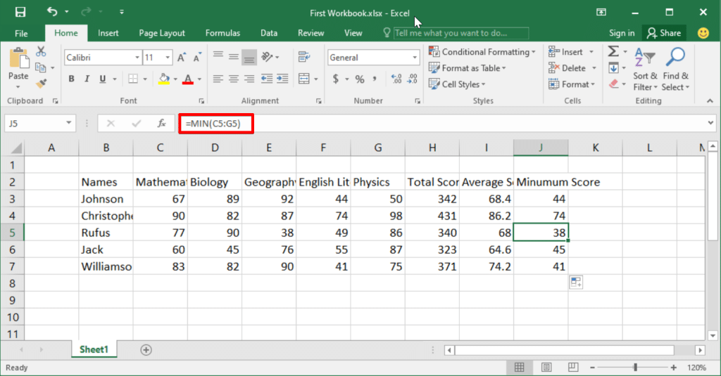
MIN/MAX: They return the minimum and maximum values respectively in a specified range. Let’s add a minimum score column.

These are some of the basic functions you can use while analyzing data in Excel. Some more advanced Excel functions include:

• VLOOKUP: The VLOOKUP function allows you to search for a value in the first column of a table and return a specific value from a different column in the same row. For instance, =VLOOKUP(“John”, A1:C10, 2, FALSE) searches for “John” in column A and returns the corresponding value from column B.
• SUMIFS and SUMIF: These functions help you sum values based on specific criteria. For instance, =SUMIF(A1:A10, “>5”, B1:B10) sums values in the range B1 if the criterion “>5” in the range A1 is met.The SUMIFS function, on the other hand, allows multiple criteria: =SUMIFS(B1:B10, A1:A10, “>5”, C1:C10, “<100”) sums the values in B1 if A1 is greater than 5 and C1 is less than 100.
• OFFSET: You can use the OFFSET function to return a cell or range of cells with a defined number of rows and columns from the specified reference cell. For example, =OFFSET(A1, 2, 3) returns the cell at two rows down and three columns to the right of A1, which is D3.
• INDIRECT: The INDIRECT function allows you to build dynamic cell references by referring to a text string representing a cell address. For instance, =INDIRECT(“A” & 2) returns the value in cell A2.

By mastering these formulas and functions, you’ll be on your way to becoming proficient in Excel and unlocking its potential for data analysis and organization.

How to Use Excel Tables and Formatting Techniques

How to Create a Table in Excel

In Excel, tables play a crucial role in organizing and analyzing data. They help you organize your information in a structured format that can be easily analyzed

Let’s create one from our scores data:

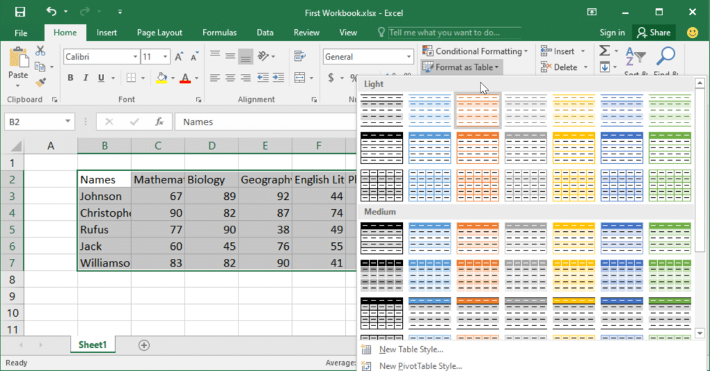
• Select all the cells with data and click Format as Table on the Home tab.
• You can choose from a variety of predefined table styles to suit your needs.

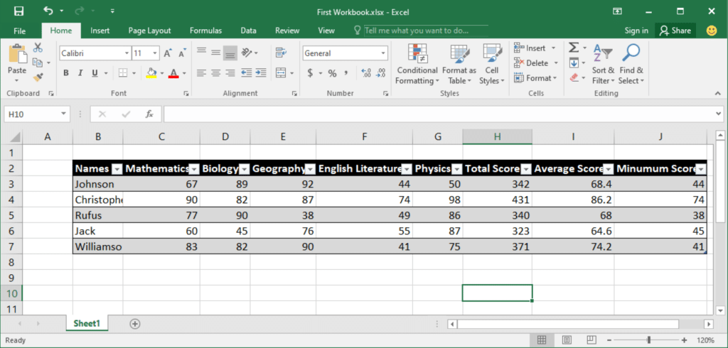
• Since our table has headers, we’re going to make sure that the My table has headers box is ticked.
• Once you have a table, you can easily sort and filter the data by clicking on the drop-down arrows in the headers, allowing you to quickly analyze your data.

Excel Table Formatting Techniques

Now that you’ve created your table, you need to format it so it looks aesthetically pleasing. Excel offers multiple formatting techniques that can enhance the appearance and readability of your tables. Some important techniques include

1. Resizing Columns and Rows: Adjust column width or row height to fit your data neatly. You can manually drag the line separating two columns, use the double-click autofit method, or set specific column widths/row heights using the Home tab.Let’s autofit all the columns so they fit all the data.
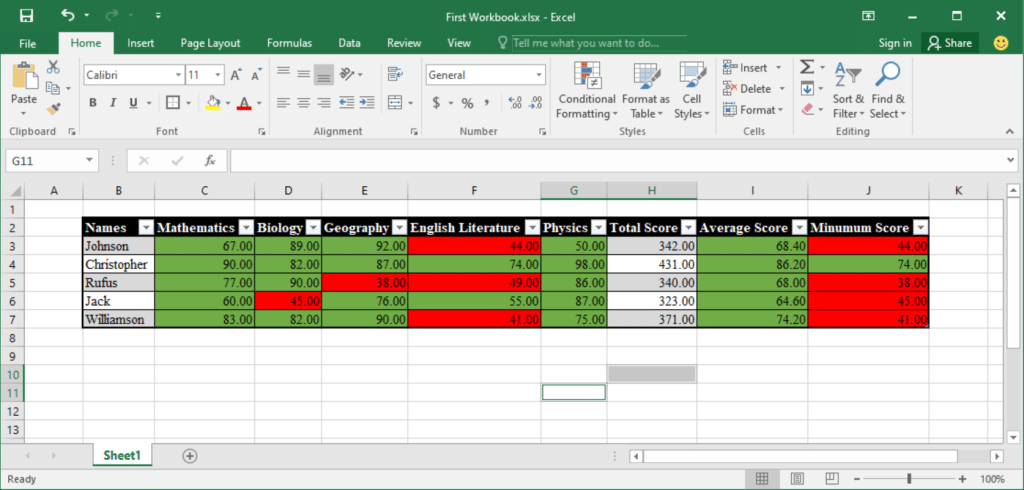
2. Conditional Formatting: It allows you to automatically apply specific formatting (like bold text, background color, or font color) based on particular cell values or conditions. To apply conditional formatting, select the desired cells, go to the Home tab, and click Conditional Formatting.We’re going to display cels with scores above 50 in green and those below in red.
3. Cell Formats: Excel allows you to define the format of cells (e.g., general, number, date, currency). To apply specific cell formats, select your desired cells, right-click on them, and choose Format Cells. Let’s format all our scores as numbers with two decimal places.
4. Using Filters: Filters can help you simplify the process of sorting and analyzing data. By applying filters to your table headers, you can quickly view subsets of data based on specific criteria. Click the drop-down arrow in the header and select your filter options.

Here’s our final table:

There are several more Excel table functions that you cnBy mastering these formatting techniques, you’ll be able to create polished, user-friendly tables. Don’t forget to practice and experiment with these features to become more knowledgeable about them.

How to Visualize Data Through Charts In Excel

Learning Excel quickly involves understanding one of its key features: data visualization through charts. This allows you to create visually appealing presentations of your data, making it easier to analyze and understand.

Basics of Creating Charts

To get started with data visualization in Excel, you need to familiarize yourself with the basic process of creating charts. Here are some steps to help you create your first chart:

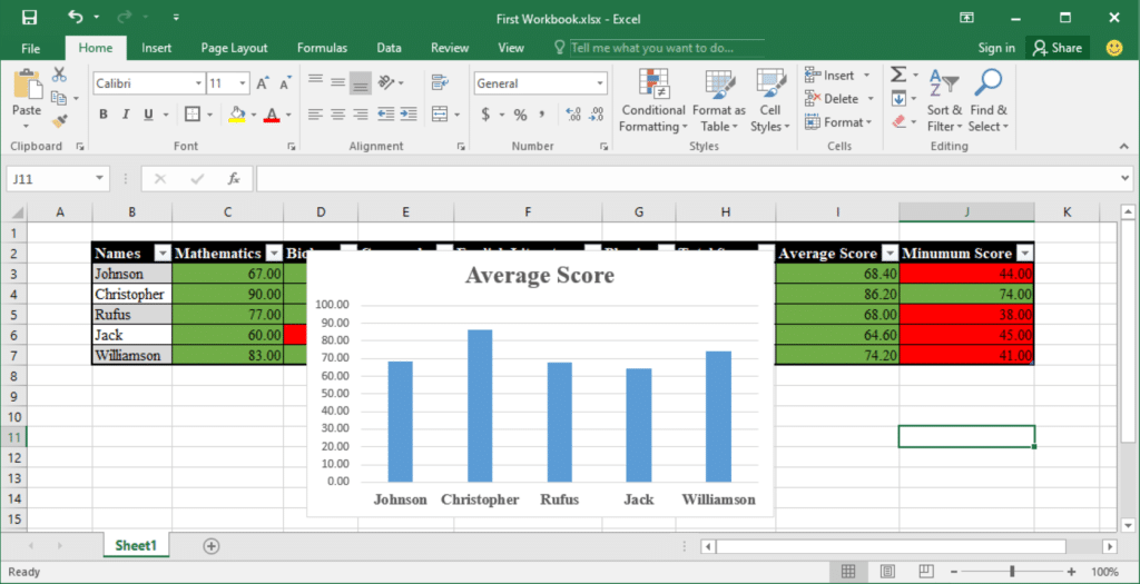
1. Select data: Choose the cells containing the data you want to visualize by clicking and dragging to select them. Let’s create a bar chart using our Name column and the Average column
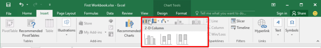
2. Choose chart type: Click the ‘Insert‘ tab, and then select the desired chart type from the ‘Charts’ group (e.g., column, bar, line, or pie). Let’s use the 2D Column chart option.

1. Customize chart: Use the ‘Design‘ and ‘Format‘ tabs to modify the chart’s appearance, such as changing colors, fonts, and labels.
2. Insert chart: Click ‘OK’ to insert the chart into your worksheet. You can reposition and resize it as needed.

Remember to experiment with different chart types to find the best visualization for your data. For example, a stacked bar chart may provide more insight into the types of data we have available here.

Advanced Chart Techniques in Excel

Once you’ve mastered the basics, you can enhance your data visualization skills by exploring advanced chart techniques. Some useful visualizations you can create include:

• Dashboards: Combine multiple charts and other elements (e.g., slicers or buttons) to create a comprehensive, interactive dashboard that provides a summary of your data at a glance.
• Sparklines: These are tiny charts that fit inside individual cells and serve as a compact visual representation of trends in your data. To create a sparkline, go to the ‘Insert’ tab and select ‘Sparklines’ from the ‘Sparklines’ group, then choose the data and target cell.
• Conditional formatting: Apply this technique to highlight specific data points or trends in your chart. For example, you can use color scales to emphasize high and low values in a range or icons to indicate the performance of a specific metric.
• Dynamic charts: Make your charts automatically update when the underlying data changes by using formulas or Excel tables as the chart’s source data. This ensures that your data visualization remains up-to-date and accurate.

By mastering these Excel data visualization techniques, you can quickly create clear and compelling charts that showcase your data’s important trends and insights.

How to Create Pivot Tables in Excel

A pivot table is a powerful Excel tool that lets you analyze and summarize your data to discover insights and trends within it. In this section, you will learn more about creating Pivot Tables to effectively analyze your data in Excel.

Creating Your First Pivot Table

To create your first Pivot Table, follow these steps:

1. Select the data range you want to analyze.
2. Go to the Insert tab in the ribbon.
3. Click on the Pivot Table button.
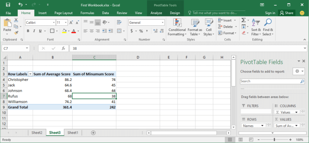
4. In the Create Pivot Table dialogue box, choose where to place the Pivot Table.

Now that you have your Pivot Table created, you can start analyzing you data with it. You can drag and drop drop fields to the Rows, Columns, and Values areas. This will allow you to analyze your data based on different factors easily.

How to Print a Spreadsheet in Excel?

When you have completed your work in Excel and you’re ready to print, follow these steps for proper printing:

1. Save your Excel file by clicking ‘Save As‘ from the File menu and selecting your preferred file format
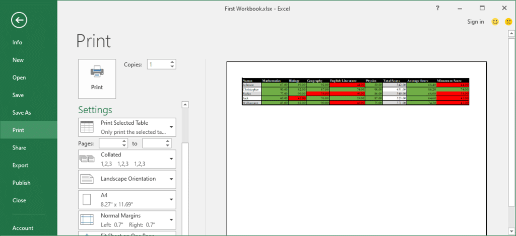
2. Click on ‘Print‘ from the File menu or press Ctrl + P as a shortcut
3. In the Print settings, adjust the desired print options, including:
   • The orientation (portrait or landscape)
   • Scaling
   • Print area selection
   • Margins and more
4. Click ‘Print Preview‘ to see how your spreadsheet will look when printed
5. If everything looks good, click ‘Print‘

How to Use Templates in Excel

One way to quickly become proficient in Microsoft Excel is to use pre-made templates. These templates are designed by experts and can save you time by providing a ready-to-use layout, formatting, and even formulas.

You can find many Excel templates by simply browsing through Microsoft Excel’s template library or downloading from online resources. By using these templates, you can learn from existing layouts and formulas and discover new features and functions while speeding up your work.

To access pre-made templates in Excel, follow these steps:

1. Open Excel and click on ‘New’ from the File menu
2. Explore the available templates, or search for a specific template with a keyword

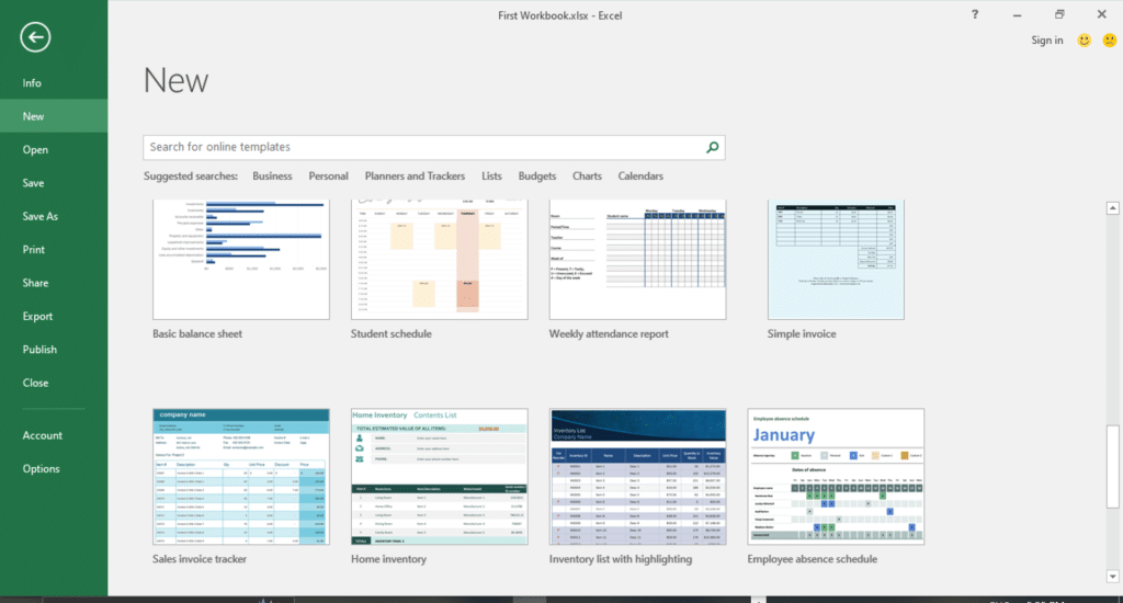
3. Click on your desired template and then Excel will download it and place it in a workbook.

How to Collaborate On and Share Spreadsheets in Excel

Sharing Spreadsheets in Excel

Sharing Excel spreadsheets has never been easier than with OneDrive or SharePoint, making it simple for you and your colleagues to access files when needed. To share a spreadsheet, follow these steps:

1. Ensure that you are signed into your Microsoft 365 account in Excel.
2. Save your file to SharePoint Online or OneDrive.
3. Click the ‘Share’ button in the top-right corner of the Excel window.

You’ll be prompted to enter the email addresses of the users you want to share the file with. Alternatively, you can also generate a link to your spreadsheet, which you can share with your colleagues or team members.

Remember that storing your file on OneDrive or SharePoint ensures that updates are saved in real time and can be accessed by the intended audience. You can learn more about Sharing Excel files in this video on How To Refresh An Excel File In Sharepoint With Power Automate Desktop.

How to Work Collaboratively in Excel

Thanks to the co-authoring feature, working collaboratively in Excel has become more efficient. The co-authoring feature allows multiple users to concurrently work on the same Excel workbook, which significantly streamlines group projects.

To work collaboratively on a spreadsheet, you and your team would need to use the OneDrive or SharePoint version of the file. Once the file is shared and opened by all collaborators, the changes each person makes will be visible to everyone in a matter of seconds.

To better manage tasks and responsibilities, you could:

• Assign tasks: Use comments to assign tasks to your team members, and resolve comments once the tasks are completed.
• Track changes: Excel provides a real-time presence feature that shows updates made by collaborators, making it easy to stay aware of any changes being made.
• Stay organized: Leverage the power of Excel’s formatting capabilities, such as tables, conditional formatting, and filters, to keep your team’s collaboration focused and efficient.

By utilizing Excel’s sharing and collaboration functionalities, you can optimize teamwork, ensure effective communication, and solve problems more quickly. This, in turn, translates into an accelerated learning curve and a better grasp of Excel’s many features.

Final Thoughts

Mastering Excel skills can prove to be invaluable in both your personal and professional life.

By now, you should have a solid understanding of how quickly and effectively you can learn how to use this powerful tool.

As you refine your Excel skills, you’ll unlock the potential to make data-driven decisions and increase efficiency in your day-to-day tasks!

If you want a handy guide to help you as you embark on your Excel journey, be sure to check out our Excel Cheat Sheet: A Beginners Guide With Time-Saving Tips.

Frequently Asked Questions

Which Excel tutorials are suitable for beginners?

For beginners, it’s essential to start with basic tutorials that cover the fundamentals of Excel. There are many free and paid Excel courses that you can use when learning these fundamentals.

Microsoft offers online courses for various skill levels, including entry-level content. You can also access many free templates and other resources from this course.

How can I master Excel formulas quickly?

The best way to learn Excel is to focus on understanding the logic behind each formula and practice using them in various scenarios. Break down complex formulas into smaller parts, and learn the core functions first, such as SUM, AVERAGE, COUNT, and IF.

As you gain confidence, progress to more advanced functions like VLOOKUP, INDEX, and MATCH.

Are there any free Excel courses with certification?

While there are plenty of free Excel courses online, most certifications require a fee. That said, sometimes you can find limited-time promotions or discounts on certification exams. Microsoft offers official certifications like the Microsoft Office Specialist (MOS) for Excel, but these typically come at a cost.