
One of Microsoft Excel’s powerful features is using formulas to do calculations and changes to data in different cells. Commonly, you must use the same formula on multiple cells simultaneously.
There are multiple ways to apply the same formula to multiple cells in Excel, including the Fill Handle, Copy and Paste, and Keyboard Shortcuts.
The Fill Handle method allows you to input the formula in the initial cell and drag the fill handle across the cells.

The Copy and Paste function allows you to manually select and duplicate the formula in desired cells.
Finally, the Keyboard Shortcut allows you to enter the formula, use ‘Ctrl+C’ to copy, then select the desired cells and press ‘Ctrl+V’ to paste.
In this article, we’ll show you how to apply the same formula to multiple cells using the above methods.
We’ll also explore different ways to work with ranges and selections, advanced techniques using Excel functions, handling data types, and automating tasks.
Let’s get into it!

Getting Started with Excel Formulas
Excel is a powerful spreadsheet software that helps you to organize, analyze, and manipulate data. One of the primary tools for handling data in Excel is formulas.

In this section, we’ll discuss the basics of Excel formulas, focusing on cell references and types of Excel formulas.
1. Understanding Excel Cell References
Before diving into Excel formulas, it’s essential to understand cell references.
In Excel, a cell reference refers to the address or location of a cell in the spreadsheet. Excel uses a combination of letters and numbers to identify cells.
The letter corresponds to the column, and the number corresponds to the row.
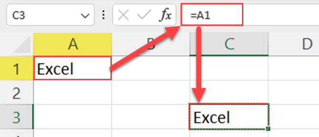
For example, the cell reference A1 refers to the cell in column A and row 1.
There are two types of cell references in Excel:
Relative Cell References
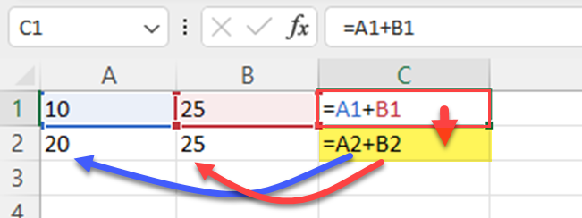
The default reference type, where the reference changes as you copy the formula across cells.
For example, if you have a formula in cell C1, =A1 + B1, and copy it to cell C2, Excel will update the cell references to =A2 + B2.
Absolute Cell Reference
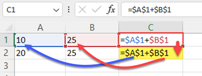
Anchors the reference, so it doesn’t change when the formula is copied.
Absolute references use a dollar sign ($) before the row and/or column.
For example, =$A$1 + $B$1.
2. Types of Excel Formulas
Formulas in Excel are equations that perform calculations using the values in the cells. There are various types of formulas in Excel, including:
1) Arithmetic Formulas
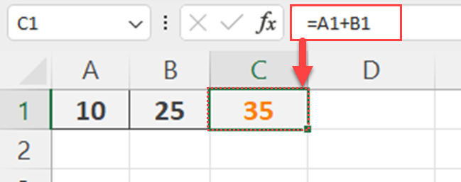
These formulas use basic arithmetic operators (+, -, *, /) to perform calculations.
Example: =A2 + B2
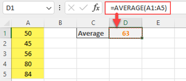
2) Statistical Formulas
Excel provides a wide range of statistical functions (e.g., AVERAGE, SUM, COUNT) to analyze data.

Example: =AVERAGE(A1:A5)
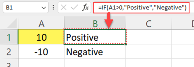
3) Logical Formulas
These formulas enable you to make decisions based on certain conditions (e.g., IF, AND, OR).
Example: =IF(A1>0, “Positive”, “Negative”)
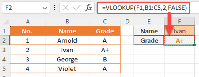
4) Lookup Formulas
Lookup and reference formulas (e.g. XLOOKUP, VLOOKUP, HLOOKUP, INDEX, MATCH) enable you to search for and retrieve specific information from data tables.
Example: =VLOOKUP(F1,B1:C5,2,FALSE)
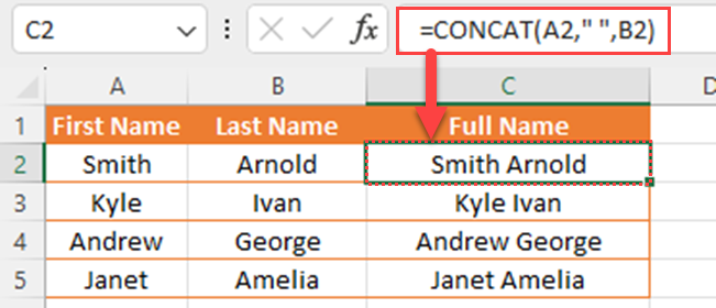
5) Text Formulas
Text formulas help you manipulate text strings in cells (e.g., CONCAT, LEFT, RIGHT, TRIM, TEXTBEFORE, TEXTAFTER).
Example: =CONCAT(A2, ” “, B2)
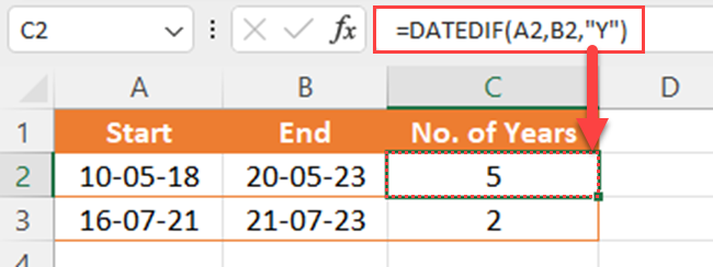
6) Date And Time Formulas
These formulas work with dates and times to perform calculations (e.g., TODAY, NOW, DATE, WEEKDAY).
Example: =DATEDIF(A1, B1, “Y”)
Applying the Same Formula to Multiple Cells
Applying the same formula to multiple cells in Excel can save time and reduce errors when working with large datasets.
This section will cover three simple methods to achieve this: Using the Fill Handle, Using Copy and Paste, and Keyboard Shortcuts.
1. Using the Fill Handle
The Fill Handle is a small square located at the bottom-right corner of a selected cell in Excel.
This handy feature helps you to quickly copy the formula from one cell to adjacent cells in the same row or column.
To apply the same formula using the Fill Handle, you can follow the steps given below:
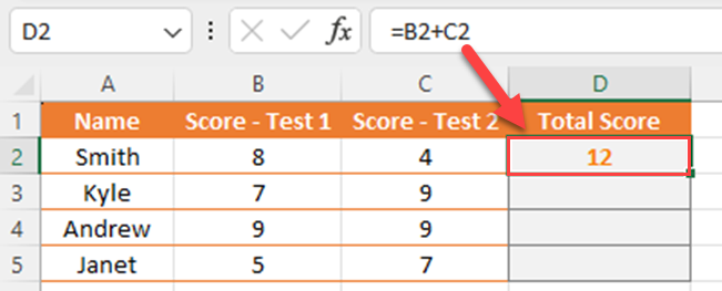
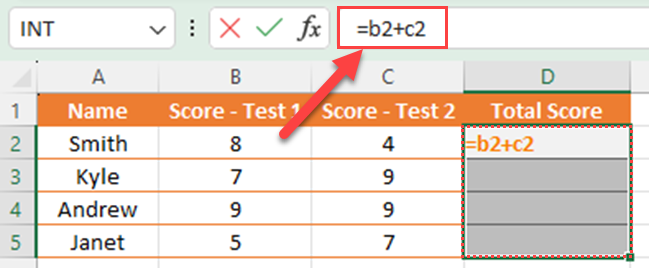
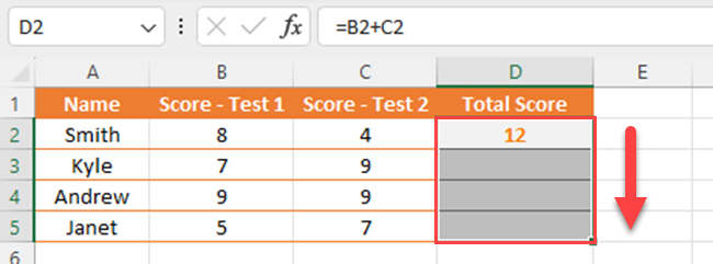
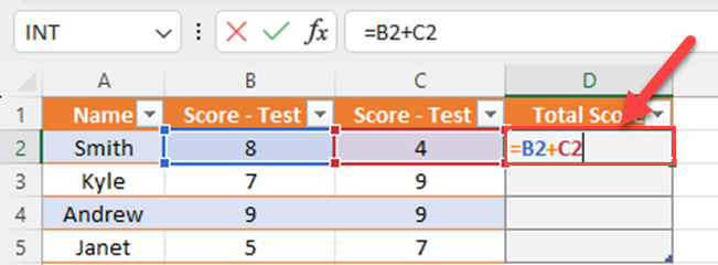
1) Click on the cell containing the formula you want to apply to multiple cells.

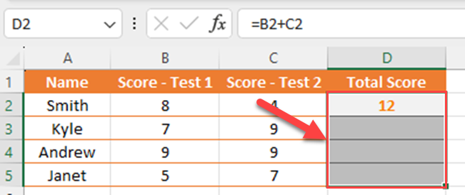
2) Position your cursor over the Fill Handle (the small square at the bottom-right corner of the selected cell).
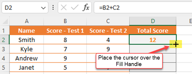
3) Click and drag the Fill Handle either up or down, left, or right, depending on the direction in which you want to apply the formula.
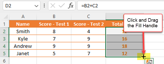
4) Release the left mouse button when you have covered the desired range of cells.
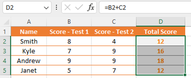
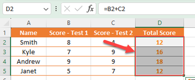
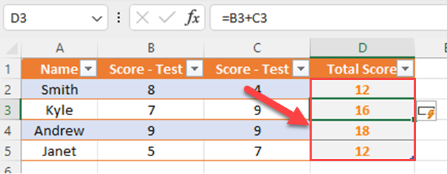
Excel will now automatically adjust the cell references in the copied formula to suit the new location, saving you time and effort.
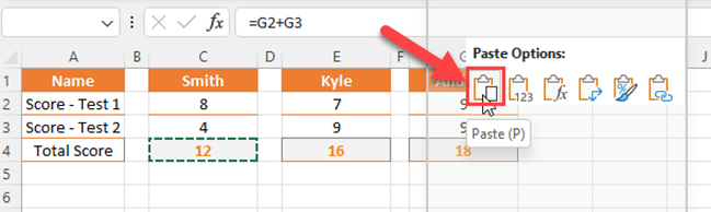
2. Using Copy and Paste
Another method to apply the same formula to multiple cells is by using Copy and Paste.

To apply the same formula to multiple cells, you can follow the steps given below:
1) Click on the cell containing the formula you want to copy.
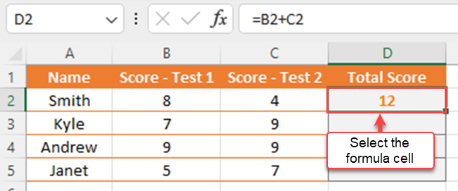
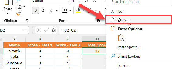
2) Press Ctrl+C (or right-click and select Copy) to copy the cell contents.
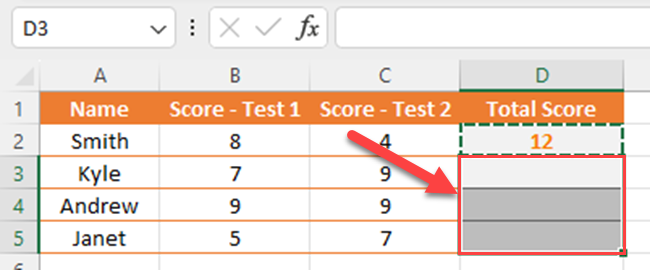
3) Select the range of cells where you want the formula to be applied.
4) Press Ctrl+V (or right-click and select Paste) to paste the formula into the selected cells.
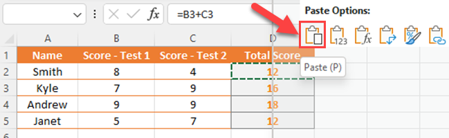
Excel will ensure that the cell references are updated as needed in the copied formula.
3. Keyboard Shortcuts
Applying the same formula to multiple cells can be even faster by using keyboard shortcuts in Excel.
You can follow the steps given below to apply the same formula to multiple cells in Excel:
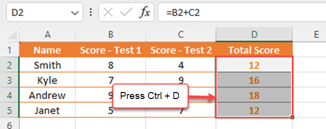
1) Enter the formula you want to apply to multiple cells in a single cell (You’ll see the formula in the formula bar).
2) Select the range of cells where you want to apply the formula, including the cell with your initial formula.
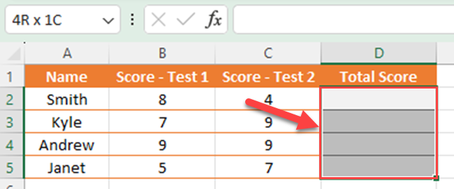
3) Press Ctrl+D to fill the formula down a column or Ctrl+R to fill the formula to the right in a row to all selected cells simultaneously.
Another way to apply the same formula to multiple cells is by using the Ctrl keyboard shortcut.
You can follow the steps below for that:
1) Select multiple cells where you want to apply the same formula.
2) Type the formula that you want to apply.
3) Press “Enter” while holding down the “Ctrl” key.
By applying these methods, it’s possible to fill multiple cells with the same formula efficiently, streamlining your workflow and increasing your productivity in Excel.
Working with Ranges and Selections
In this section, we’ll discuss different ways to work with ranges and selections in Excel to apply the same formula to multiple cells.
1. Selecting Adjacent Cells
Selecting adjacent cells is a common task when working with formulas.
To apply a formula to adjacent cells, follow these steps:
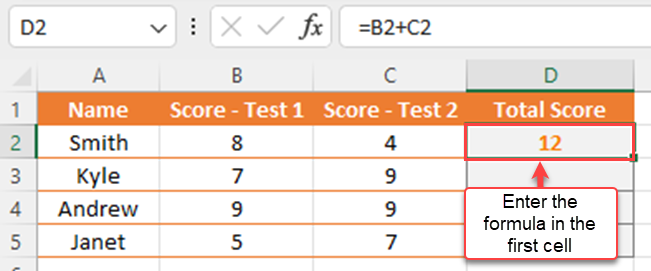
1) Enter the formula in the first cell of the range.
2) Select the cell containing the formula. Then, position the cursor over the fill handle.
3) Click and drag the fill handle (the small square at the bottom-right corner of the cell) across the adjacent cells you want to apply the formula.
Alternatively, you can use keyboard shortcuts by following the steps given below:
1) Press Ctrl + Enter to apply the formula to all selected cells.
2) Press Ctrl + R to copy the formula to the right.
3) Press Ctrl + D to copy the formula down.
2. Selecting Non-Adjacent Cells
Applying a formula to non-adjacent cells requires a different approach.
You can execute this by following the steps below:
1) Enter the formula in the first cell.
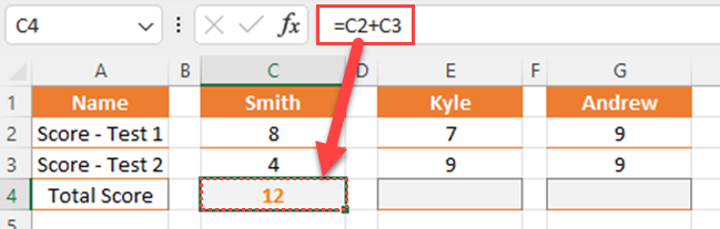
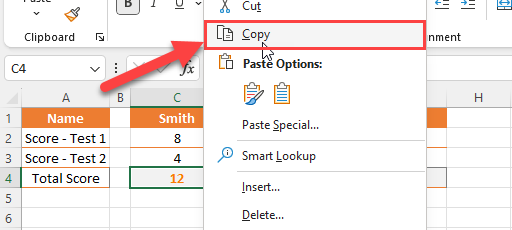
2) Select the cell containing the formula and press Ctrl + C to copy it (or right-click and select Copy).
3) Holding the Ctrl key, click on the non-adjacent cells where you want to apply the formula.
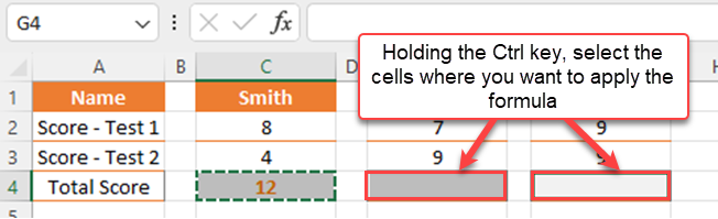
4) Press Ctrl + V (or right-click and select Paste) to paste the formula into the selected cells.
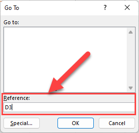
3. Using the Go To Feature
The Go To feature in Excel is a powerful tool that helps you quickly navigate to specific cells or ranges based on certain criteria.
To use the Go To feature, press F5 or Ctrl + G to open the Go To dialog box.
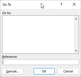
From here, you can:
1) Enter a specific cell address and press Enter or click the OK button to go directly to that cell.
2) Click the Special button to select cells based on criteria such as:
- Formulas
- Constants
- Blank cells
- Errors
Advanced Techniques for Copying Formulas
In this section, we’ll explore some advanced techniques to apply the same formula to multiple cells in Excel.
The methods covered here are Using Ctrl + Enter and Ctrl + R, Applying Formulas to Excel Tables, and Converting to Range.
1. Using Ctrl + Enter and Ctrl + R
This keyboard shortcut is a quick way to apply a formula to multiple cells simultaneously.
You can follow the steps below to apply a formula to multiple cells:
- First, select the desired range of cells.
- Next, write the formula in the active cell (usually the top-left cell).
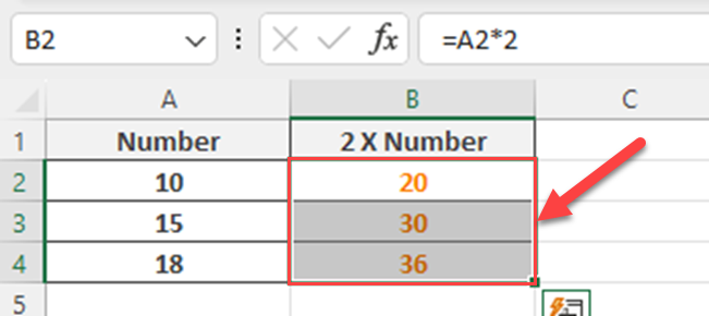
- Then, press Ctrl + Enter.
This will apply the same formula to all the selected cells.
Here’s a quick example:
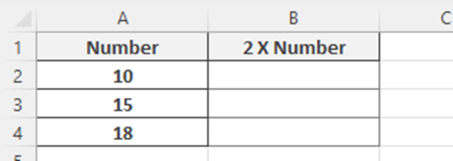
To multiply values in column A with 2 and get the output in column B:
1) Select the cells in Column B where you want to apply the same formula.
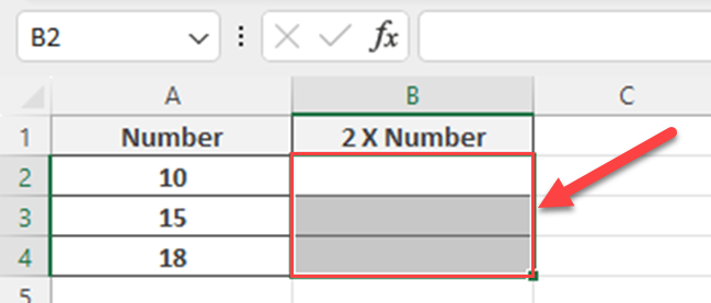
2) Type =A2*2
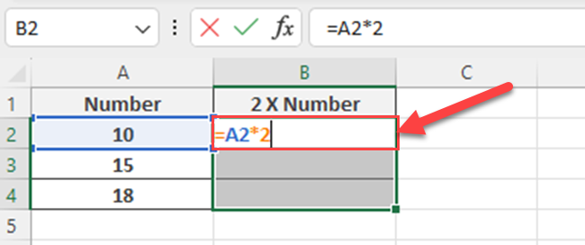
3) Press the Control Key and Enter Key together
If you want to apply a formula horizontally to adjacent cells, you can use the Ctrl + R keyboard shortcut.
2. Applying Formulas to Excel Tables
Excel tables are a robust method for managing and analyzing data. When you insert a formula in an Excel table, it automatically fills the entire table column.
Here is how to apply formulas in an Excel table:
1) Convert the data to an Excel table by selecting the range, and press Ctrl + T.
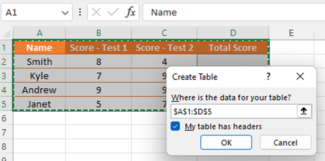
2) Type the formula in the desired cell within the table.
3) Hit Enter and the formula will automatically apply to the entire column.
When you want to apply the same formulas for multiple columns, you have to repeat the above steps for each column.
3. Converting to Range
If you want to remove the table formatting and convert an Excel table to a normal data range, you can follow the steps listed below:
1) Select any cell within the Excel table.
2) Go to the Table Design tab, which appears when you select a table cell.
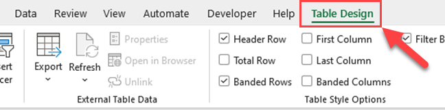
3) Click Convert to Range in the Tools group.
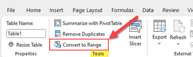
This will remove the table formatting and features, such as automatic formula filling.
Your data will now be in a normal range, and you can apply formulas using the above methods or any other desired technique.
Using Functions in Excel
Excel provides a wide range of functions to simplify calculations and data handling.
This section focuses on using these functions to apply the same formula to multiple cells.
1. Common Functions
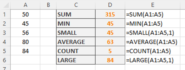
Below are some commonly used functions in Excel:
- SUM: Calculates the sum of a range of cells (=SUM(A1:A5)).
- MIN: Returns the smallest number in a range of cells (=MIN(A1:A5)).
- SMALL: Finds the nth smallest value in a data set (=SMALL(A1:A5, 1) for the smallest value).
- AVERAGE: Calculates the average of a range of cells (=AVERAGE(A1:A5)).
- COUNT: Counts the number of non-empty cells in a range (=COUNT(A1:A5)).
- LARGE: Finds the nth largest value in a data set (=LARGE(A1:A5, 1) for the largest value).
- QUARTILE: Calculates the specific quartile for a given data set (=QUARTILE(A1:A5, 2) for the second quartile).
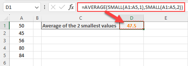
2. Combining Functions
Excel allows you to combine functions to create more complex formulas. To achieve this, you can nest one function within another.
Below, you’ll find 2 examples of combining functions in Excel.
1) Calculating the average of the two smallest values in a range: =AVERAGE(SMALL(A1:A5, 1), SMALL(A1:A5, 2))
2) Calculating the sum of a range, excluding lowest value: =SUM(A1:A5)-MIN(A1:A5)
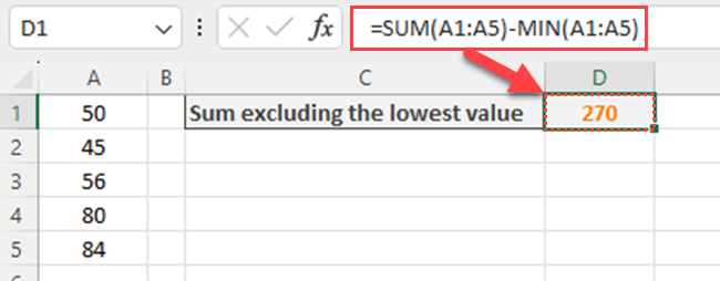
By using the appropriate combination of functions, you can handle diverse data sets and do various tasks in Excel with ease.
Handling Different Data Types
Consistency in data types is important when working with data. In this section, we will explore how you can handle different data types in Excel.
1. Working with Currencies
When working with currencies in Excel, it’s crucial to ensure that the correct currency format is applied to the data.
This can be done in the following ways:
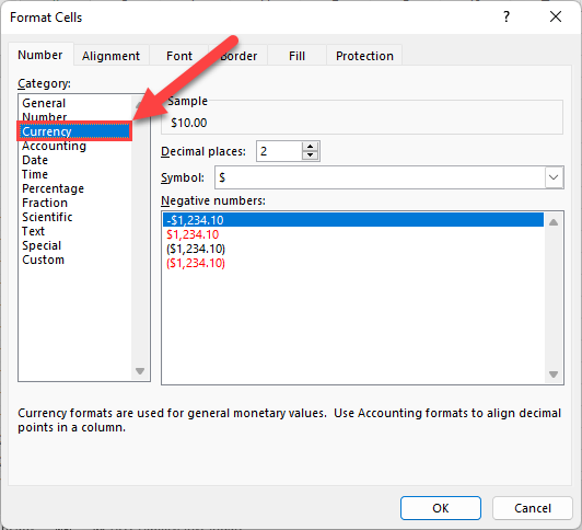
- Selecting the desired cells, right-click, and select “Format Cells”.
- In the “Number” tab, choose “Currency” and select the appropriate currency symbol (e.g. USD, GBP, EUR, JPY).
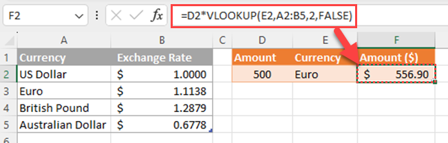
To do calculations with different currencies, it’s necessary to use exchange rates.
To convert a value from one currency to another, you can use the VLOOKUP function to find the exchange rate in the table, then multiply the value by the corresponding rate:
=D2*VLOOKUP(E2,A2:B5,2,FALSE)
2. Calculation Based on Data Types
When performing calculations on different data types, it’s important to ensure that the data is properly formatted.
For example, when calculating fees or other currency values, ensure that the data is stored in a column with the correct currency format.
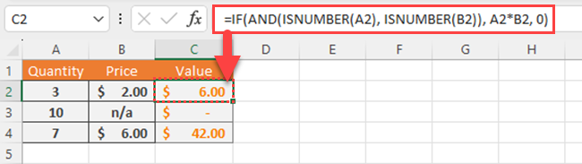
Here’s an example formula for calculating the product of values in columns A and B and placing the result in column C:
=IF(AND(ISNUMBER(A2), ISNUMBER(B2)), A2*B2, 0)
This formula checks if the product of the values in cells A1 and B1 can be calculated.
If not, it displays “0” in the corresponding cell in column C.
When handling different data types in Excel, always ensure that the data is correctly formatted and use appropriate functions to perform calculations.
Automating Excel Tasks
Automation lies at the heart of efficient computing.
In this section, we will explore how you can automate your Excel tasks such as applying the same formula to multiple cells.
Specifically, we will talk about the following:
- Using Autofill and Autocomplete
- Using Visual Basic for Applications (VBA)
1. Using Autofill And Autocomplete
Autofill and Autocomplete are two built-in features in Excel that can help you save time when applying the same formula to multiple cells.
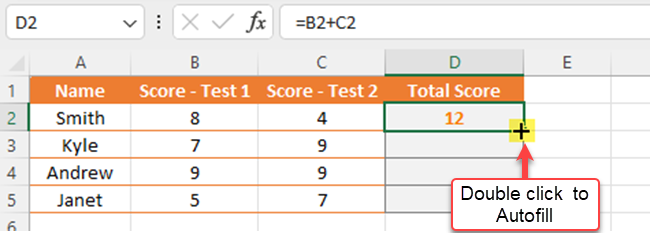
Autofill is a feature that automatically fills in a series of values based on a pattern or formula.
To use autofill, simply enter your formula in the first cell, then click on the small square in the bottom right corner of the cell and drag it across or down the desired range of cells.
Autocomplete is another handy feature that predicts and displays possible entries as you type, based on previous values entered in the same column.
This can be especially useful when you’re working with a lot of data and need to enter similar information repeatedly.
To use Autocomplete, start typing in a cell and Excel will provide suggestions based on previous entries in the same column.
Press Enter or Tab to accept the suggested entry.
2. Using Visual Basic for Applications (VBA)
Visual Basic for Applications (VBA) is a powerful programming language built into Excel, which allows you to automate tasks and create custom functions.
VBA can be used to apply the same formula to multiple cells on an Excel sheet.
To get started with VBA, follow these steps:
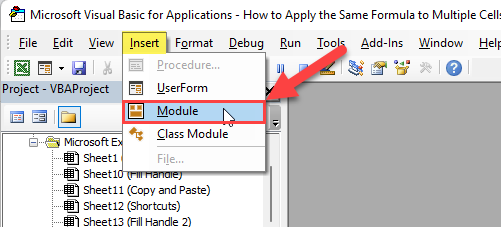
1) Press Alt + F11 to open the Visual Basic for Applications window.
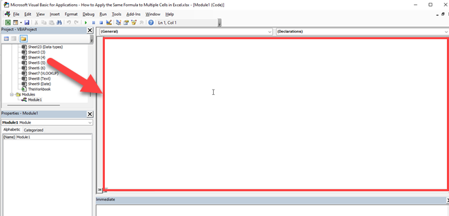
2) Click Insert in the menu, then select Module to create a new module for your code.
3) In the module, you can write your VBA code or macro.
For example, you can create a simple VBA code to apply the same formula to a range of cells:
Sub ApplyFormula()
    Range("B1:B10").Formula = "=A1*2"
End Sub
This VBA code applies the formula =A1*2 to cells B1 to B10. To run the code, press F5 or go to the menu Run > Run Sub/UserForm.
Using VBA can significantly enhance your Excel experience, enabling you to automate repetitive tasks, create custom functions, and streamline your workflow.
Learn more about DAX & Excel Formulas by watching the following video:
Final Thoughts
In summary, learning how to apply the same formula to many cells in Excel is a valuable skill for working with data.
The methods explored in this article help save time and prevent mistakes, making your work easier and more organized.
Incorporating these techniques into your Excel routine empowers you to efficiently manage large datasets.
Whether you’re a student, professional, or dealing with numbers regularly, these skills enhance productivity and accuracy in Microsoft Excel.
Frequently Asked Questions
In this section, you’ll find some frequently asked questions that you may have when applying formulas to multiple cells in Excel.

How to drag the formula down?
Yes, you can quickly apply a formula to multiple cells by dragging it down.
After typing the desired formula in the first cell, click on the bottom-right corner of the cell (highlighted square), and drag it down to the adjacent cells.
The formula will be applied to all the cells as you drag it.
How to apply the formula to a whole column?
To apply a formula to the entire column, you can use the keyboard shortcut Ctrl+D.
First, type the formula in the topmost cell, then select the entire column (including the cell with the formula) and press Ctrl+D.
This will fill the selected column with the formula.
How to copy the formula with changing references?
When you copy a formula in Excel, relative references will change according to their new location.
For example, if you have a formula “=A1+B1” in cell C1 and copy it to C2, the formula will update to “=A2+B2.”
However, if you want to keep the original references, you can use absolute references by adding a $ symbol before the row or column reference, e.g., “=$A$1+$B$1”.
How to apply multiple formulas in one cell?
It is not possible to have multiple formulas in one cell in Excel.
Each cell can only contain one formula or value.
To perform multiple operations or use multiple formulas, you can break them down into separate cells or combine them into a single formula using Excel functions and operators.
How to lock formulas in multiple cells?
To prevent accidental changes or deletion of formulas in multiple cells, you can lock them.
First, select the cells you want to lock, right-click and choose “Format Cells.”
In the “Protection” tab, check the “Locked” option, and click “OK.”
Next, go to the “Review” tab and click “Protect Sheet,” enter a password (optional), and click “OK.”
How to use the same cell in formulas?
To use the same cell reference in multiple formulas or cells, you can use absolute references by adding a $ symbol before the row or column reference.
For example, if you want to use cell A1 in multiple formulas, you can write the formula as “=$A$1+”.
This will ensure that it always refers to cell A1, even if you copy or move the formula to other cells.


