
Excel SUMIF function is a very powerful function that helps you to sum cells based on criteria. This function is particularly useful when dealing with large datasets, as it helps you to get the SUM of the actual cells that meet the criteria.
The SUMIF function syntax is SUMIF(range, criteria, [sum_range]). The “range” is the cell range to be evaluated, “criteria” means the specific condition to be met, and the optional “sum_range” indicates the cells to be summed if the criteria are met. The function can handle various criteria types, including numerical values, text criteria, and even dates.
In this article about Excel’s SUMIF function, you’ll learn a multitude of concepts that can transform the way you work with data. We’ll begin by explaining what SUMIF is, its syntax, and its purpose within the Excel ecosystem. You’ll learn how to use SUMIF to conditionally sum cells based on single or multiple criteria and distinguish the difference between SUMIF and SUMIFS.

Let’s get started!

Understanding the Excel SUMIF
The Excel SUMIF is a useful built-in function that allows you to sum values in a range based on specific criteria. This function is widely employed for summing cells that fulfill certain conditions, like values based on dates, text, or numbers.
1. Basic Usage
With the SUMIF, you can perform calculations on data that meet the given criteria. For example, if you have a column containing numbers and you want to sum only the values larger than 5, you would use the following formula:
=SUMIF(B2:B8,”>5″)
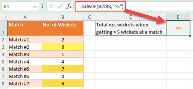
This formula sums all values in the range B2 to B8 that are strictly greater than 5. It’s important to remember that the SUMIF function only works with a single condition. If you need to apply multiple conditions, you have to use the SUMIFS function.
2. Syntax
The Excel SUMIF function has three arguments: range, criteria, and sum_range:

=SUMIF(range, criteria, [sum_range])
- range: This is the cell range that you want to apply the criteria to. In the range argument, you can include a number, text, or date range.
- criteria: The criteria or condition that decides which cells to include in the sum. Criteria can be entered as text, numbers, or cell references.
- sum_range (optional): The cell ranges to sum. If this argument is not provided, the SUMIF formula will add cells in the specified range.
For example, if you wish to sum all values in column A (A1) that are less than or equal to 10, use the below formula with the following arguments:
=SUMIF(A1:A5, “<=10”)
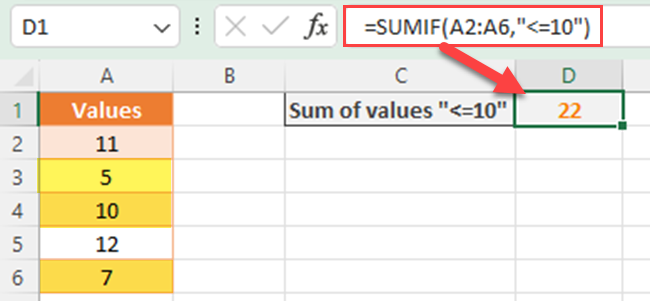
It’s important to write the criteria using the correct syntax. For example, a criterion using a greater-than sign (>) should be enclosed in double quotation marks, like this: “>5”.
With a better understanding of Excel SUMIF, you can confidently use it to do calculations on specific data based on your criteria. This function is an essential tool in Excel that helps make data analysis more efficient and effective.
Working With Criteria Using SUMIF in Excel
In this section, we’ll explore the concept of working with criteria using the SUMIF function in Excel.
One of Excel’s most useful features is its ability to perform complex calculations and apply conditions to these calculations.
The SUMIF function is particularly useful in this regard, as it allows you to sum data that meet criteria you specify, hence offering a great deal of flexibility.
1. Single Condition
When using the SUMIF in Excel, you can sum cells in a range based on a single condition (criteria) such as dates, text string values, or numbers. The basic syntax for SUMIF is:
=SUMIF(range, criteria, [sum_range])
- range: The range of cells to be evaluated by the criteria.
- criteria: The condition to be met for cells to be included in the sum.
- sum_range: An optional argument for the range of cells to be added. If omitted, the cell range given in the range argument will be used.
For example, if you want to sum the values in column A that are greater than 10, you would use =SUMIF(A1:A10, “>10”).
2. Multiple Criteria Using SUMIFS
If you need to evaluate multiple criteria, you can use the SUMIFS function. The syntax for SUMIFS is:
=SUMIFS(sum_range, criteria_range1, criteria1, [criteria_range2, criteria2],…)
- sum_range: The range of cells to be added.
- criteria_range: The range of cells to be evaluated for each criterion.
- criteria: The conditions to be met for cells to be included in the sum.
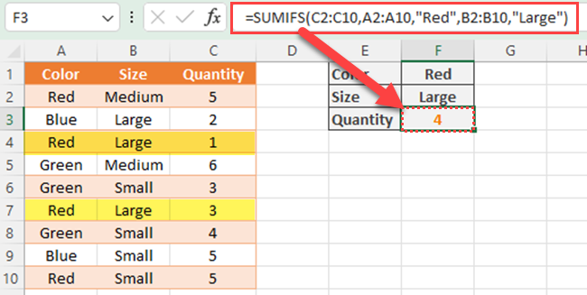
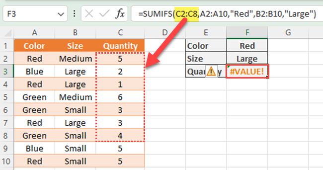
For example, if you want to sum values in column C for rows where column A has “Red” and column B has “Large”, you would use =SUMIFS(C2:C10, A2:A10, “Red”, B2:B10, “Large”) like in the following example.
3. Logical Operators
When defining criteria in SUMIF or SUMIFS, you can use logical operators such as “=”, “<>”, “>”, “>=”, “<“, and “<=”. These operators allow for more complex criteria evaluations, as shown in the previous examples.

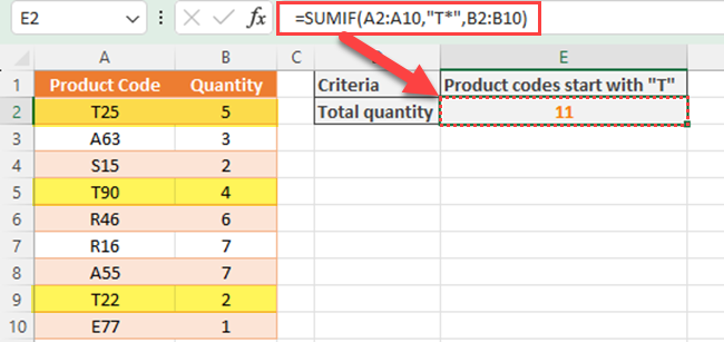
4. Wildcard Characters
In Excel SUMIF and SUMIFS functions, you can use wildcard characters for text criteria. The main wildcard characters are:
- ?: Matches any single character.
- *: Matches any sequence of characters.
For example, to sum values in column B where the corresponding cells in column A start with “T”, you can use the below formula:
=SUMIF(A2:A10, “T*”, B2:B10).
Handling Different Data Types With SUMIF
When working with Excel’s SUMIF function, it is important to be mindful of handling different data types. In this section, we’ll discuss the proper handling of numbers, dates, and text for the SUMIF function.
1. Numbers
SUMIF is designed primarily to handle numbers. When defining the criteria for the function, you should specify the range of cells (range) and the criteria to be evaluated.
The sum_range argument is optional, and if omitted, the function will use the same range argument and sum range. Cells within the specified ranges should contain numbers, names, arrays, or references that contain numbers:
=SUMIF(range, criteria, [sum_range])
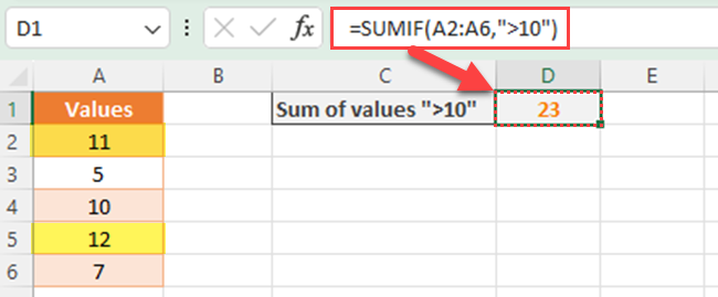
For example, to sum only the values in column A greater than 10, you can use the SUMIF formula like this:
=SUMIF(A2:A6,">10")
2. Dates
Similar to numbers, dates can also be utilized within the SUMIF function. To handle dates, ensure that cells within the range contain valid date formats (mm/dd/yyyy or dd/mm/yyyy). You can use SUMIF to evaluate and sum up a range of cells based on certain date criteria.
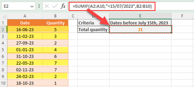
If you want to sum the values in column B for entries with dates before July 15th, 2023, use the following SUMIF formula:
=SUMIF(A2:A10,"<15/07/2023",B2:B10)
3. Text
SUMIF can also use text-based criteria. Although the primary purpose of this function is to handle numbers, it can evaluate cells containing text values. In such cases, the text-based criteria need to fulfill certain conditions for the sum calculation.
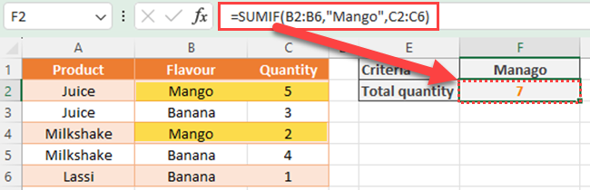
For example, if you want to sum the values in column C for entries where column B contains the text “Mango”:
=SUMIF(B2:B6,"Mango",C2:C6)
Always ensure that the data types in your range and criteria are consistent to achieve accurate results using the SUMIF function.
Common Examples and Use Cases of SUMIF
Excel’s SUMIF function is an indispensable tool for many business applications, especially when dealing with financial or sales data. It allows you to sum values in a specified range based on a set of criteria.
In this section, we’ll cover some common examples and use cases, showcasing the versatility and power of the SUMIF function.
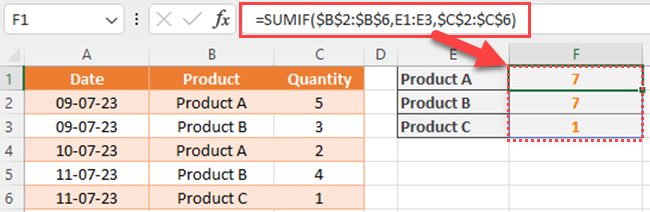
Suppose you have a list of sales data with date, product, and sales amount columns, and you want to calculate the total sales of a specific product. You can use the following formula:
=SUMIF(B2:B6,”Product A”,C2:C6)
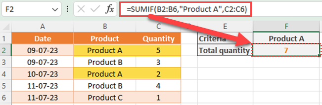
This formula will sum the sales amounts in the range C2 to C6, where the corresponding product name in column B matches “Product A”.
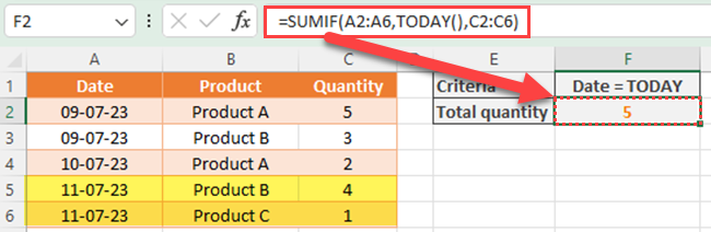
If you want to find the total sales for today, you can insert the TODAY() function into the SUMIF criteria for the date column. Then, your formula is:
=SUMIF(A2:A6, TODAY(), C2:C6)
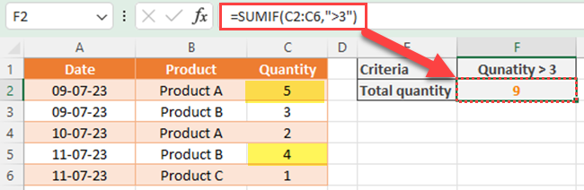
For example, when you need to sum values based on greater than or less than criteria, SUMIF can also be used. Let’s say you want to find the total sales for products with a sales quantity greater than 3. You can achieve this with the following formula:

=SUMIF(C2:C6,”>3″)
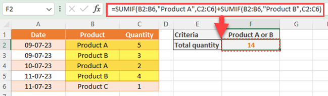
SUMIF can also be combined with OR logic using the addition of multiple SUMIF functions. For example, if you want to calculate total sales for “Product A” or “Product B”, you can use this formula: =SUMIF(B2:B6,”Product A”,C2:C6) + SUMIF(B2:B6,”Product B”,C2:C6)
Keep these examples in mind when you use the SUMIF function to work with your data, as its versatility helps simplify complex calculations and streamline financial analysis. Remember to be confident, knowledgeable, and clear when working with this function to maximize the benefits it can provide.
Dealing With Errors and Troubleshooting SUMIF in Excel
When working with the SUMIF function in Excel, you might encounter errors or challenges. In this section, we’ll discuss some common issues and their solutions.
1. #VALUE! Error
One common error when using the SUMIF function is the #VALUE! error. This can occur due to the following reasons.
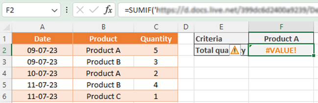
- SUMIF function returns #VALUE! error if SUMIF has a cell reference or a range in a closed workbook. The solution is to open the closed workbook that contains cell references and refresh the formula.
- If you are trying to match text strings of more than 255 characters in SUMIF formulas, you’ll get a #VALUE! error. To resolve this issue, try shortening the string if possible. If not, use the CONCATENATE function or the Ampersand (&) operator to break down the value into multiple strings.For example: =SUMIF(B2:B12,”long string”&”another long string”).
- SUMIFS function inconsistency: In some cases, the criteria_range argument within the SUMIFS function may not be consistent with the sum_range argument. To fix this, ensure both arguments reference the appropriate ranges and that both ranges have the same dimensions.

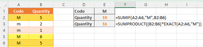
2. Case-Sensitive Criteria
If your data is case-sensitive, the SUMIF function may not produce accurate results, as it is not case-sensitive by default. In such situations, consider using the SUMPRODUCT function, which supports case-sensitive criteria.
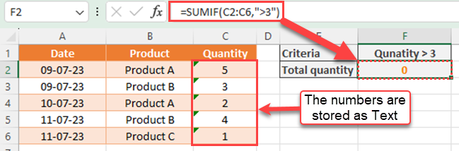
3. Returning a zero value
If the SUMIF function isn’t working as expected and returns a value of zero, check the following:
- Ensure that there are no syntactical errors in the formula.
- Verify that the range contains the correct data types (numbers or references that contain numbers).
- Make sure the condition or criteria specified is accurate and complete.
4. Dealing With Multiple Conditions
If you need to apply more than one condition while summing values, the SUMIFS function is an excellent choice. This function allows multiple criteria to be specified across different ranges. Be sure to use accurate ranges and criteria while implementing the SUMIFS function.
By addressing these common issues and troubleshooting properly, you can effectively use the capabilities of Excel’s SUMIF and SUMIFS functions to sum values with specific criteria.
Advanced Techniques and Customization Using SUMIF
In this section, we’ll learn some advanced techniques and customization options for the Excel SUMIF function that can expand its capabilities and improve efficiency in managing large datasets.
1. Using SUMPRODUCT With SUMIF
The SUMPRODUCT function can be used with SUMIF to perform conditional calculations. This approach is especially useful when dealing with datasets containing multiple criteria.
For example, if you want to calculate total sales for “Product A” or “Product B”, you can use this formula:
=SUMPRODUCT(SUMIF(B2:B6,{“Product A”,”Product B”},C2:C6))
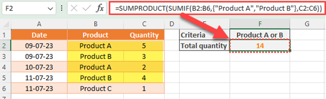
This makes it easier to analyze your data and compare sales figures across different regions.
2. Array Formulas
An array formula is a more advanced way to use Excel functions that allow you to perform multiple calculations simultaneously. With the SUMIFS function, you can combine array formulas to calculate the total quantity for each product. In other words, you can enter a criteria range.
This can save time and effort by reducing the need for multiple steps in your calculations.
3. Excel 365 Features
Users of Excel 365 can leverage the UNIQUE and SUMIFS functions together for more advanced data analysis. This combination allows for quick and easy calculation of total invoice values per customer, without the need for additional steps or complex formulas.
4. Evaluating Conditional Statements
When using advanced techniques with SUMIF, it’s important to be aware of how Excel evaluates conditional statements. For instance, using “<” (less than), “<=” (less than or equal to), or “>=” (greater than or equal to) can help you filter and calculate results based on specific conditions.
This can be particularly useful when analyzing data with a wide range of values and understanding how different data points or ranges contribute to your overall analysis.
By mastering these advanced techniques and customizations in Excel SUMIF, you can elevate your data analysis skills to a higher level.
Remember to always apply these methods thoughtfully and with a clear understanding of the desired outcome, as inaccurate calculations can lead to misleading results and misguided decision-making.
Compatibility With Different Excel Versions
The SUMIF function is a versatile and commonly used function found in different versions of Microsoft Excel. This section discusses its compatibility across various Excel versions, including 2010, 2013, 2016, 2019, and 2021.

1. In Excel 2010, the SUMIF function works efficiently to perform calculations based on specific criteria. However, updates in December 2010 caused ActiveX control issues which impacted the functionality of some Excel features. This can be resolved by deleting all *.exd files present in the system folders, thus ensuring smooth functioning.
2. Excel 2013 introduced the SUMIFS function, which is an improved version of SUMIF that allows for multiple criteria to be used. The original SUMIF function still functions as expected in Excel 2013. Users can leverage the updated functionality with the SUMIFS function when working with multiple conditions.
3. In Excel 2016 and Excel 2019, the SUMIF and SUMIFS functions are both available and fully functional. The syntax and usage remain consistent across these versions, allowing users to perform calculations with one or multiple criteria.
4. Excel 2021 continues to maintain compatibility with the SUMIF and SUMIFS functions, ensuring that users can utilize them for calculations across a wide range of Excel versions.
In conclusion, the SUMIF function is compatible with various Excel versions, including Excel 2010, 2013, 2016, 2019, and 2021. The more advanced SUMIFS function was introduced in Excel 2013 and is fully functional in subsequent versions.
Final Thoughts
The SUMIF function in Excel proves to be an incredibly powerful tool for analyzing and summarizing data. Its ability to sum values based on specific criteria brings a new level of flexibility and sophistication to data management tasks.
Over the course of this article, we’ve covered the basics of the SUMIF function, delving into its syntax, examining various examples, and demonstrating how to effectively handle and troubleshoot common issues.
As we wrap things up, it’s important to note that SUMIF is just one of many powerful functions in Excel’s toolkit. There’s a wealth of other functions and features available, waiting to be harnessed to meet your unique data processing and analysis needs!
If you’d like to learn more about Excel functions, check out the video below:
Frequently Asked Questions
How do you use Sumif with multiple conditions?
To use SUMIF with multiple conditions, you need to use the SUMIFS function. The syntax is as follows: =SUMIFS(sum_range, criteria_range1, criteria1, [criteria_range2, criteria2], …). This allows you to provide several criteria that must be met for the cells to be included in the sum.
What is the difference between Sumif and Sumifs?
The main difference between SUMIF and SUMIFS is that SUMIF can only handle a single condition, while SUMIFS can handle multiple conditions. The syntax for SUMIF is =SUMIF(range, criteria, [sum_range]), while the syntax for SUMIFS is =SUMIFS(sum_range, criteria_range1, criteria1, [criteria_range2, criteria2], …).
How to use Sumifs with multiple sheets?
To use SUMIFS with multiple sheets, you need to use INDIRECT or SUMPRODUCT functions, referring to the different sheets’ ranges. Here is an example of the SUMIFS function used with two sheets: =SUMIFS(INDIRECT(“Sheet1!” & sum_range), INDIRECT(“Sheet1!” & criteria_range1), criteria1, INDIRECT(“Sheet2!” & criteria_range2), criteria2). This formula will sum the values in sum_range of Sheet1 if they meet the criteria1 and criteria2 from Sheet1 and Sheet2, respectively.
Can Sumif and Vlookup be combined?
Yes, SUMIF and VLOOKUP can be combined to achieve more complex calculations. This can be done by embedding a VLOOKUP function within a SUMIF function. The syntax would look like this: =SUMIF(criteria_range, VLOOKUP(lookup_value, criteria_lookup_range, index_number, [range_lookup]), sum_range). This formula will sum the values in sum_range if they meet the criteria obtained from the VLOOKUP function.
How to sum cells containing text?
Unfortunately, SUMIF alone cannot sum cells containing text, as it is designed to work with numeric values. However, you can use other functions, such as IF and COUNTIF, combined with the original cell values, to sum cells containing specific text.
How to use If and Sumif together?
You can nest the IF function within the SUMIF function to achieve more complex calculations with additional conditions. The syntax for this would be: =SUMIF(range, IF(condition, criteria, alternative_criteria), [sum_range]). This formula will sum the values in sum_range if the cells in the range meet the specified criteria for the given condition. If the condition is not met, it will use the alternative criteria.


