8 Ways To Add Specific Cells in Excel

One of the most common tasks in Excel is adding specific cells together. This can be as simple as adding two individual cells or more complex, like summing cells that meet certain criteria.

Fortunately, Excel offers a variety of built-in functions and tools to help you achieve this. In this article, you’ll learn how to add specific cells in Excel using eight different methods.

By understanding these techniques, you will quickly become more proficient in handling data.

Ok, let’s get into it.

How to Select Specific Cells To Add Together

Before you can add specific cells in Excel, you’ll need to select them properly. This can be done in at least four ways:

• Using keyboard keys.

• Using the Name Box.

• Using named ranges.

• Using data tables.

1. Keyboard Keys

The keys to use differ between Windows and Mac Excel. If you’re using Windows, you can click on each cell individually while holding the Ctrl key. On Mac Excel, hold the Command key down.

This is useful for selecting non-contiguous cells. The method can be tedious if you have a lot of cells, but there’s a shortcut if you’re working with a continuous range.

To select a continuous range of cells:

1. click on the first cell in the range

2. hold down the Shift key (Windows) or Command key (Mac Excel)

3. click on the last cell in the range.

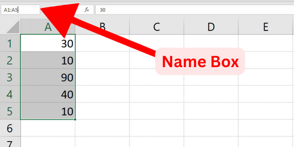
2. Using the Name Box

The Name Box is located in the upper-left corner of the worksheet. You can manually type in the cell reference range (for example, A1:A5).

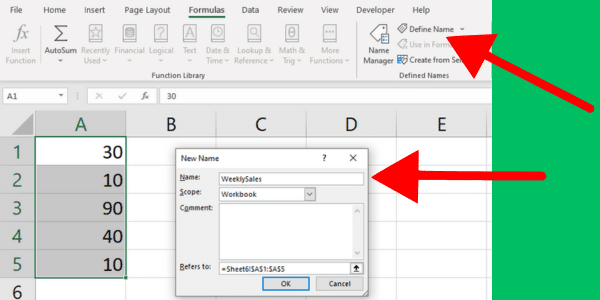
3. Using Named Ranges

If you find yourself frequently typing the same range, you can use named cells or ranges to make your formulas easier to read and manage. To define a named range:

1. select the cells first

2. go to the Formulas tab

3. click on Define Name

4. Using Data Tables

Data tables in Excel can help you add large amounts of data. To create a data table with the cells you want to add:

1. Select a range of cells containing your data, including headers

2. Click on the “Table” button in the “Insert” tab

3. Make sure the “My table has headers” checkbox is selected, and click “OK”

Now that you know these ways to select specific cells in Windows and Mac Excel, the following methods will let you add the values.

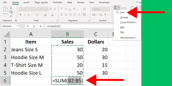
1. Using Excel’s Autosum Feature

The Autosum command is a built-in feature in Excel that allows you to quickly and easily calculate the sum of selected cells.

The Autosum button is located on the Home tab of the Excel ribbon, in the Editing group.

Follow these steps:

1. Select the cell where you want the sum to appear.

2. Click on the AutoSum button in the Editing group on the Home tab.

Excel will automatically try to determine the start and end of the sum range. If the range is correct, press Enter to apply the sum.

If the range is not correct, you can drag your mouse over the range of cells you wan, and then press Enter to apply the sum.

This first example shows the command summing the value of total sales:

You can also use the Autosum command across a row as well as a column. Highlight the cells in the row, choose where you want to calculate the result, and press the button.

2. Using the Excel SUM Function

You can easily add specific cells in Excel by using the SUM function. This operates on all the cells you specify.

Here is how to add specific cells in Excel using SUM():

1. Type =SUM( in a cell, followed by an opening parenthesis (.

2. Select the first cell or range to be added, for example: A1 or A1:A5.

3. If you want to add more cells or ranges, type a comma, to separate one argument from the next.

4. Select the next cell or range, such as B1 or B1:B5.

5. Continue adding cells or ranges separated by commas until all cells have been included in the formula.

6. Close the parenthesis with ) and press Enter to complete the formula and get the sum.

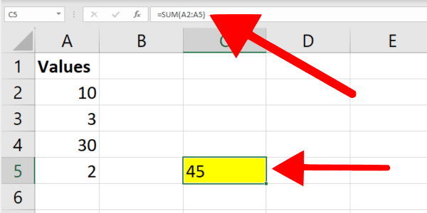
The result will sum values in all the cells specified. This picture shows the sum of cells A1 to A5:

Remember that the cells you’re including in the formula don’t have to be adjacent. You can add any cells in any order.

For example, if you want to add cells A2, B4, and C6, this is the SUM formula:

=SUM(A2, B4, C6)

3. Addition By Cell Reference

You can also sum cells based on their cell references. This method is particularly useful when you want to add only a few particular cells in Excel that fit specific criteria.

To do this, follow the steps below:

1. Choose one cell to display the result and type an equals sign (=).

2. Select the first cell you’d like to add by clicking on it or typing its reference (e.g., A2).

3. Enter the addition operator or plus sign (+).

4. Select the second cell you’d like to add by clicking on it or typing its reference (e.g., B2).

5. Press Enter to get the result.

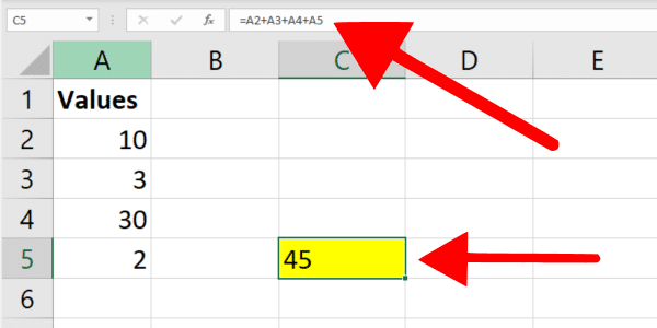
For example, if you want to add two cells A2 and B2, your formula would look like this:

=A2+B2

If you need to add more cells, simply continue adding plus signs followed by the cell references (e.g., =A2+B2+C2). This picture shows the addition of four cells:

If you’re dealing with a larger range of cells in Excel, consider using the SUM() function I showed in the previous section.

4. Conditional Summing Using The SUMIF Function

The SUMIF function in Excel allows you to calculate sums based on a single condition. This function is useful when you want to add cells within a referenced range that meet a specific criterion.

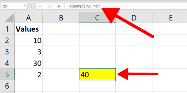
For example, suppose you want to sum cells that contain a value greater than 5. The following formula shows the syntax:

=SUMIF(A2:A5,">5")

The SUMIF function is summing all the cells in the range A2:A5 with a value greater than 5.

Here’s the step-by-step guide:

1. Select the cell where you want to display the result.

2. Type the formula containing the SUMIF function and specify the range and criteria.

3. Press Enter to complete the process.

5. Conditional Summing With The SUMIFS Function

While the SUMIF function allows you to work with a single condition, the SUMIFS function enables you to work with multiple criteria. This function is useful when you want to sum cells that meet two or more conditions.

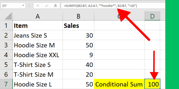
For example, suppose you want to sum cells in column B where the corresponding cells in column A contain the text “hoodie” and column B has numbers greater than 10.

The following formula shows the syntax with filtering on text values:

=SUMIFS(B2:B7, A2:A7, "*hoodie*", B2:B7, ">10")

This example formula sums the values in the range B2:B7 where the cell immediately beside them contains “hoodie” and the cells in range B2:B7 are greater than 10.

I used wildcard characters (*) to provide text filtering.

Here is how to add specific cells in Excel using multiple criteria:

1. Select the cell where you want your result to be displayed.

2. Type the SUMIFS formula mentioned above, adjusting the cell ranges and criteria as necessary.

3. Press Enter to complete the process.

Remember, both the SUMIF function and the SUMIFS function are not case-sensitive.

You can achieve even more powerful filtering if you incorporate Power Query. This video shows some of that power:

6. Using Array Formulas

An array formula is a powerful tool in Microsoft Excel for working with a variable number of cells and data points simultaneously.

First, let’s understand what an array formula is. An array formula allows you to perform complex calculations on several values or ranges at once, which means less manual work for you.

To create an array formula, you need to enter the formula using Ctrl + Shift + Enter (CSE) instead of just pressing Enter. This will surround the formula with curly braces {} and indicate that it’s an array formula.

Here is how to add specific cells in Excel using array formulas and the SUM function:

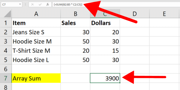
1. Select a single cell where you want the result to be displayed.

2. Type the formula =SUM(B1:B5*C1:C5) in the selected cell. This formula multiplies each value in range A1:A5 by its corresponding value in range C1:C5 and adds up the results.

3. Press Ctrl + Shift + Enter to turn this formula into an array formula.

You should now see the result of the addition in your selected cell. Remember that any changes you make to the specified cell ranges will automatically update the result displayed.

7. Using Named Ranges And The SUM Function

I showed you how to create a named range in an earlier section. Let’s now look at how to add specific cells in Microsoft Excel using a named range.

All you have to do is use the SUM function along with the named range you just created.

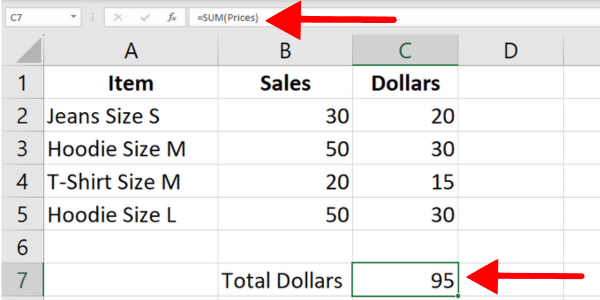
Let’s say we create a named range called “Prices” on cells C2 to C5 of our clothes data. To add the cells in the named range, enclose it within the SUM function as in the following formula:

=SUM(Prices)

You can also use the SUMIF function with a named range.

8. Using Data Tables And The SUBTOTAL Function

When you have a data table, you can use the SUBTOTAL function to add specific cells based on certain criteria.

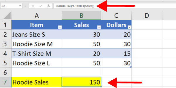
For this example, I created an Excel table from the clothes data I’ve used in previous sections. The table is named “Table1” and the first row is the header. The first column shows the items and the second column has the number of sales.

The following formula adds all the values in the sales column:

=SUBTOTAL(9, Table1[Sales])

The syntax uses the SUBTOTAL function with two arguments:

• The first argument is the function number for SUM, which is 9. This tells Excel to sum the values in the Sales column of Table1 that meet the specified criteria.

• The second argument is the range of cells to be included in the calculation, which is Table1[Sales].

Another advantage of the SUBTOTAL function is that it only includes visible cells in the specified range. In contrast, the SUM function includes both hidden and visible cells.

Combining Sums With Text Descriptions

Sometimes you’ll want to have some extra text describing the result of your summed values.

For example, when you’re using conditional summing it’s a good idea to provide some context to the numbers. To do so, you can concatenate text to the result of the calculation.

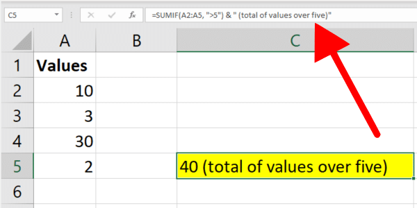
Here’s an example using the SUMIF function that is summing numbers that are higher than 5. The syntax uses the & symbol to concatenate the descriptive text.

=SUMIF(B2:B25,">5") & " (total of values over five)"

The example adds the characters after the sum. You can also add characters at the beginning of the cell.

Bonus Content: Adding Numbers In VBA

This article has focused on Excel formulas and functions. To round out your knowledge, I’ll quickly cover Excel VBA and macros.

In VBA, you add two or more numbers using the plus operator “+”. Here is some sample code:

Dim a as Integer,b as Integer, c as Integer
a = 3
b = 2
c = a + b
MsgBox "The sum of " & a & " and " & b & " is " & c

In this example, we declared three variables: a, b, and c, all of which are of type Integer. We assigned the values 2 and 3 to a and b.

Then we added a and b together using the “+” operator and assigned the result to the variable c. The last line displays the values of a and b along with the calculated sum of c.

5 Common Errors to Avoid

When working with Microsoft Excel formulas, it’s essential to avoid common errors that might lead to inaccurate results or disrupt your workflow. Here are five errors to steer clear of.

1. Incorrect Formatting

You may see a #NUM! error or a result of zero if the cells you’re working with are not formatted correctly. The problem can be with a single cell.

When cells have text values, some functions simply skip those cells. Others will show a Microsoft error code. Be sure to format your target cells as numbers.

The problem can occur when you have copied numeric data that has unsupported formatting. For example, you may have copied a monetary amount formatted like “$1,000”. Excel may treat this as a text value.

To avoid issues, enter the values as numbers without formatting. When you are copying data, you can use Paste Special to strip the formatting from the destination cell.

2. Unnecessary Merging of Cells

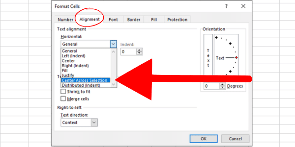
Try to avoid merging and centering cells across a row or column. This may interfere with selecting cell ranges and cause issues when working with formulas like the SUMIF function.

Instead, consider using the “Center Across Selection” option for formatting purposes. Follow these steps:

1. Select the cells

   that you want to apply the formatting to

2. Right-click on the selected cells and choose “Format Cells” from the context menu

3. In the “Format Cells” dialog box, click on the “Alignment” tab

4. Under “Horizontal”, select “Center Across Selection” from the dropdown menu

3. Incorrect Argument Separators

Depending on your location settings, you might be required to use a comma or a semi-colon to separate arguments in a formula.

For example, =SUM(A1:A10, C1:C10) might need to be =SUM(A1:A10; C1:C10) in certain regions.

Not using the correct separator can cause errors in your calculations.

4. Handling of Errors in Cell Values

When summing specific cells, it’s common for some to contain errors, such as #N/A or #DIV/0. These errors can disrupt your overall results if not handled properly.

A helpful solution is to use the IFERROR function or the AGGREGATE function to ignore or manage error values.

For instance, you can sum a range while ignoring errors by applying the formula =AGGREGATE(9,6,data), where ‘data’ is the named range with possible errors.

5. Using Criteria Without Quotation Marks

When summing cells based on criteria such as greater than or equal to specific values, be sure to enclose the criteria expression in quotation marks.

For example, when using SUMIF, the correct formula is =SUMIF(range, “>500”, sum_range), with quotation marks around the >500 criteria.

By keeping these common errors in mind and applying the suggested solutions, you can improve your Microsoft Excel skills and ensure your calculations are accurate and efficient.

Our Final Say – It’s Time For You To Excel!

You now know how to add specific cells in Excel using eight different methods and formulas. The many examples show how to sum numbers based on a selected range.

You also know how each formula works and when to use them. Each Excel formula is available in recent editions of Excel, including Excel for Microsoft 365.

Some produce the same result, while others allow different ways to filter the data on selected cells.

Best of luck on your data skills journey.

On another note, if you are looking to master the Microsft stack and take your data skills to the next level, check out our free training.