
Microsoft Excel is a powerful tool widely used for data organization, analysis, and presentation. Among its many features, one particularly useful functionality is the ability to insert hyperlinks into your spreadsheet.
To insert a hyperlink in Excel:
- Firstly, select the cell or text you want to link.
- Then, click on the “Insert Hyperlink” button or right-click and choose “Hyperlink” from the menu.
- In the dialog box, enter the URL or file path you want to link to and click “OK.
Now, the cell or text will have a clickable link leading to the specified destination.

Let’s run through it together; read on.

In this article, we’ll go over the steps to insert a hyperlink in Excel. We’ll also discuss how you can edit and remove hyperlinks, navigating hyperlinks, and hyperlink best practices.
Let’s get started!
1. Steps to Insert a Hyperlink in Excel
In this section, we’ll discuss two ways to insert a hyperlink in Excel — using the right-click menu and the insert tab. Hyperlinks streamline your navigation through Excel documents by connecting cells, web pages, addresses, and existing files.
Inserting Hyperlinks is extremely important when you are working on a large Excel workbook.
1. Using the Right-Click Menu
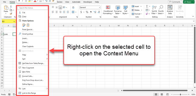
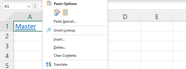
Select the cell in which you want to insert the hyperlink and Right-click on the selected cell to open the Context Menu.

1. Go to the “Link” option and click on “Insert Link.”
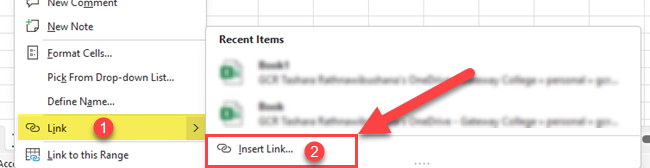
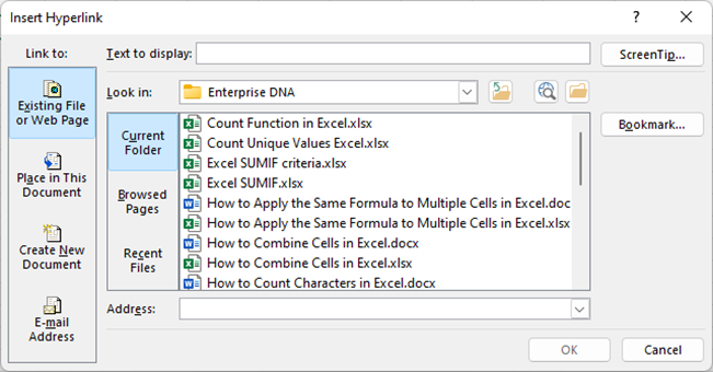
2. This action opens the “Insert Hyperlink” dialog box.
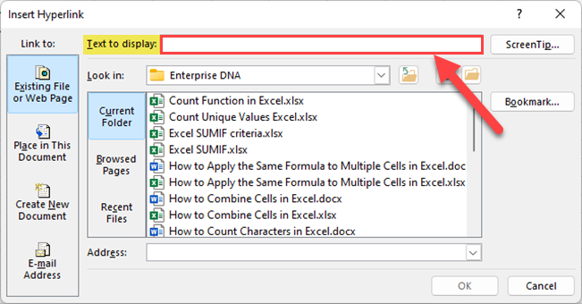
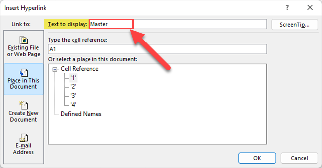
3. In the “Text to display” field, type a description that will appear as the cell content.
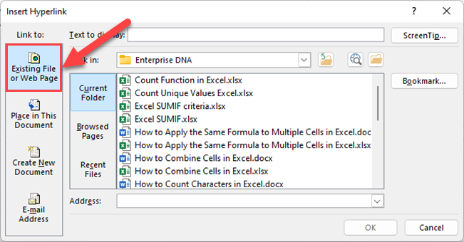
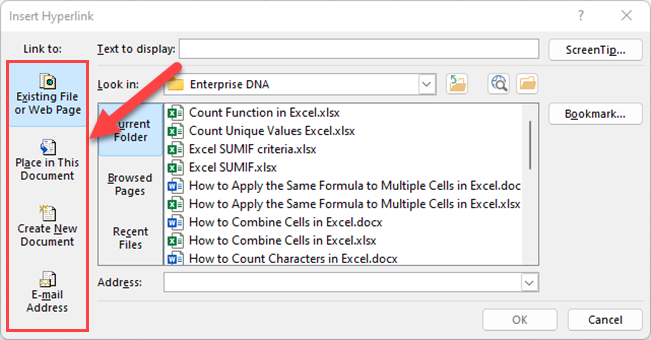
4. Choose the type of link you want to create from the following options:
- Existing file or web page: Provide the address of the file or webpage you want to link.
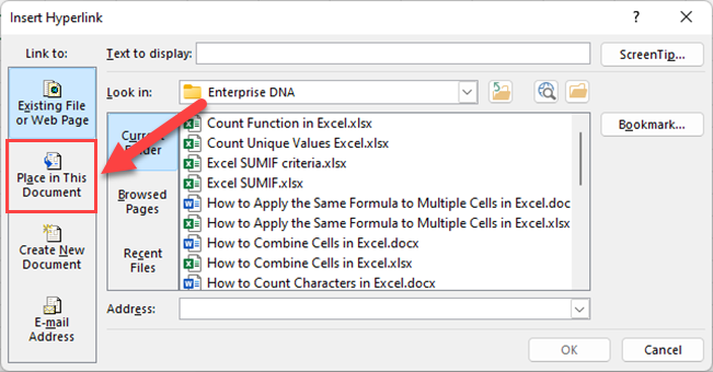
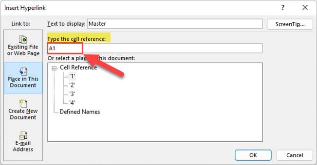
- Place in this document: Link to a specific location within your workbook by providing the cell reference.
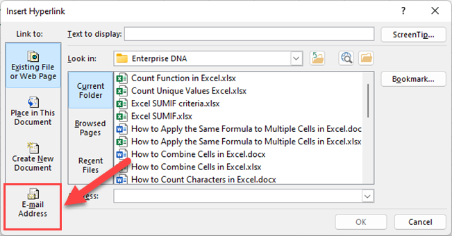
- Email address: Enter the email address that will be opened upon clicking the hyperlink.
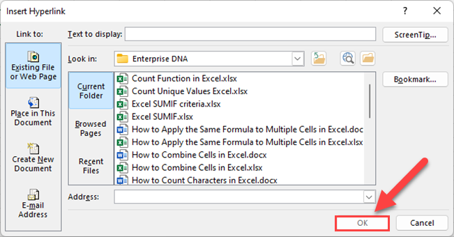
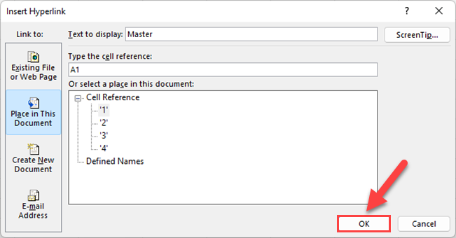
- After making your selection, click “OK” to insert the hyperlink.
2. Using the Insert Tab
To insert hyperlinks via the “Insert” tab, follow these steps:
1. Open the Excel document and select the cell in which you want to insert the hyperlink.
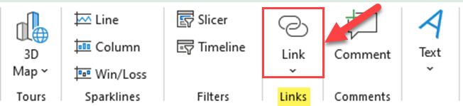
2. Go to the “Insert” tab in the toolbar.
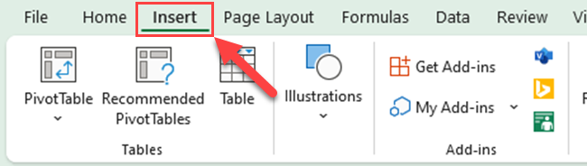
3. Go to the “Links” group and click on the “Link” icon.
4. In the “Insert Hyperlink” dialog box, type a description in the “Text to display” field to serve as your cell content.
5. Select the type of link you want to create, just as in the right-click menu method, and provide the necessary information.
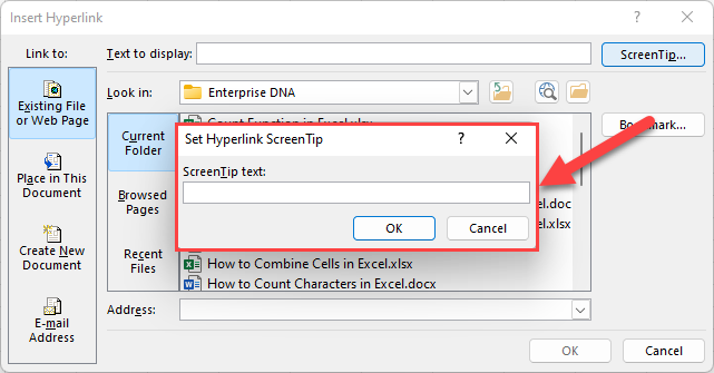
6. Optionally, you can add a “ScreenTip” for a more detailed description that appears when hovering over the hyperlink.
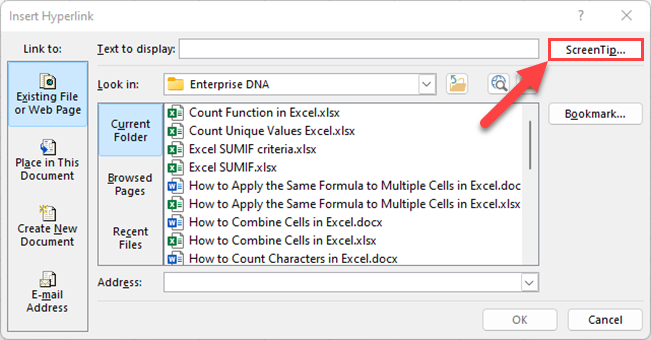
To do this, click the “ScreenTip” button, type a description in the text field, and click “OK.”
7. Finally, click “OK” to insert the hyperlink into the selected cell.
By following these simple steps, you can seamlessly insert hyperlinks in Excel to improve navigation and accessibility in your spreadsheets.
3. Using the Hyperlink Function in Excel
The Hyperlink function in Excel enables users to create and edit links to other locations, such as websites or other documents, directly within a cell.

This Excel function provides an efficient way to reference external resources and quickly go between different parts of a spreadsheet or related files.
The syntax of the HYPERLINK() function is as follows:
HYPERLINK(link_location, [friendly_name])
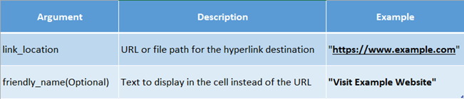
- link_location: The URL or file path of the destination. This is a required argument.
- friendly_name: Optional text that will be displayed in the cell instead of the link_location. If left blank, the link_location will be displayed.
Function Arguments
Here is a quick reference for the arguments used in the HYPERLINK() function:
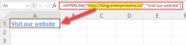
Below is an example using the HYPERLINK() function:
=HYPERLINK("https://www.example.com", "Visit Example Website")
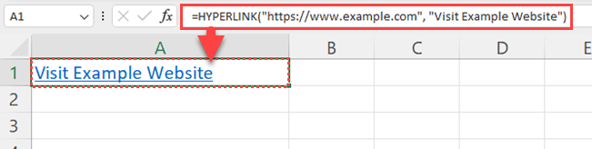
This formula will create a hyperlink to “https://www.example.com” with the displayed text “Visit Example Website”.
In summary, the Hyperlink function in Excel provides a convenient way to insert, edit, and manage hyperlinks within your spreadsheet, allowing for easy navigation and access to relevant resources.
4. Using the Hyperlink Shortcut in Excel
Sometimes you may need to quickly insert a Hyperlink in a specific cell. Then, you can use the Excel keyboard shortcut. To insert a hyperlink using this method, follow these steps:
1. Select the cell where you want to insert the hyperlink.
2. Press Ctrl + K. You have to press the Control key and the letter “K” together. Then, Excel will open the “Insert Hyperlink” dialog box.
3. Type the text that you want to show in the hyperlink in the Text to display box.
4. Type the file location/ Cell address in the cell reference box.
5. Click OK to insert the hyperlink.
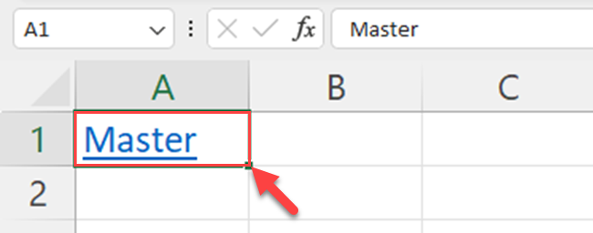
6. Then, you can see the Hyperlink with the friendly name on the selected cell. You can click the link and go to the link destination quickly.
Unlike the Hyperlink function, you can’t see the link destination cell address in the formula bar. You’ll see only the hyperlink text.
5. Applying VBA for Hyperlinks
Visual Basic for Applications (VBA) can be employed to further automate and customize the hyperlinking process:
1. Press Alt + F11 to open the VBA editor. You can also go to the “Developer” tab and press “Visual Basic” to open the VBA Editor.
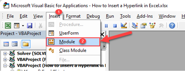
2. Go to Insert > Module to create a new module.
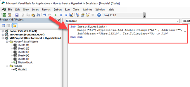
3. Type the VBA code for your desired hyperlink function. For example, the following VBA code creates a hyperlink from cell A1 to cell A10:
Sub InsertHyperlink()
    Range("A1").Hyperlinks.Add Anchor:=Range("A1"), Address:="", _
    SubAddress:="Sheet1!A10", TextToDisplay:="Go to A10"
End Sub
Remember that Microsoft 365 users have access to additional VBA functionality. Make sure to refer to the official documentation for specific features and syntax.
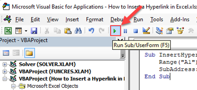
4. Press F5 or go to Run > Run Sub/UserForm to execute the code.

Now, you’ve learned different methods to create Excel hyperlinks in Excel files. It is important to know, how to edit links as well. In the next section, we’ll discuss how to edit and remove existing hyperlinks.
2. Editing and Removing Hyperlinks
First, we’ll learn how to edit hyperlinks.
1. Editing a Hyperlink
To edit a hyperlink in Excel, simply follow these steps:
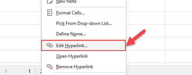
1. Right-click on the cell containing the hyperlink you want to edit. Then, Excel will open the context menu. You can even press the “Menu” key on your keyboard to open the “Context Menu”. You’ll find the “Menu” key in between the Right-side Alt key and the Right-side Ctrl key.
2. Select Edit Hyperlink from the context menu that appears.
3. In the Edit Hyperlink dialog box, you can modify the displayed text, the link’s destination, or other hyperlink options as needed.
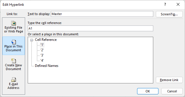
4. Click OK to apply your changes.
By following these steps, you can confidently and clearly edit the hyperlinks in your Excel worksheet.
Next, we’ll check how to remove a hyperlink from a cell.
2. Removing a Hyperlink
If you need to remove a hyperlink from your Excel worksheet, follow these steps:
1. Select the cell containing the hyperlink you want to remove.
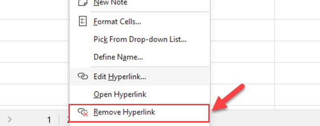
2. Right-click on the selected cell. Then, Excel will open the context menu. You can even press the “Menu” key on your keyboard to open the “Context Menu”. You’ll find the “Menu” key in between the Right-side Alt key and the Right-side Ctrl key.

3. Choose Remove Hyperlink from the context menu that appears.
Following these steps will remove the hyperlink without deleting the displayed text in the cell.
3. Navigating Hyperlinks
In Excel, you can easily insert hyperlinks to provide quick access to related information in other files, web pages, or worksheets. Navigating hyperlinks in Excel is simple and can enhance your work experience by connecting data efficiently.
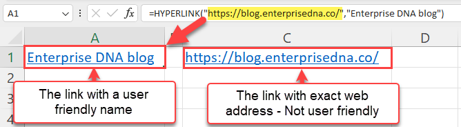
When you insert a hyperlink, you can choose the display text that appears in the cell. The display text can be different from the actual link or destination, making it more readable and meaningful to users. For example, you can display “Visit our website” as the text while linking to your company’s website address.
Clicking a hyperlink in Excel opens the destination in the default web browser if it’s an external link, such as a website. If the hyperlink is internal, pointing to another sheet within the same workbook, it will navigate to the selected sheet name instead.
To avoid accidentally activating a hyperlink when selecting a cell, simply click the cell and hold the mouse button until the cursor turns into a cross.
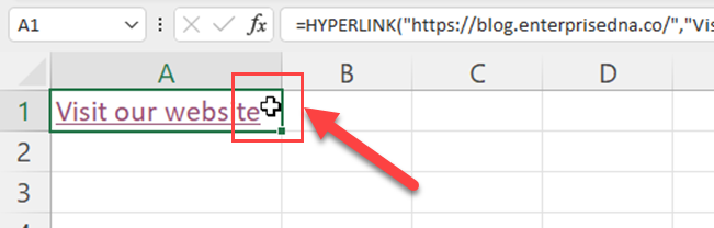
Then, release the mouse button and you can safely select and work on the cell without triggering the hyperlink.
Remember, navigating hyperlinks in Excel can significantly improve the organization and communication of your work by providing easy access to relevant external and internal resources in just one click.
4. Hyperlink Best Practices
When working with hyperlinks in Excel, it’s essential to keep a few best practices in mind to ensure that your links are effective and functional.
First, it’s a good idea to create meaningful, descriptive names for your hyperlinks. By using the friendly_name parameter in the HYPERLINK function, you can provide a clear, easy-to-understand name for your links. This will make it easier for your readers or collaborators to quickly identify the purpose of each link.
Next, consider the appearance of your hyperlinks. To maintain a consistent look throughout your workbook, apply a uniform style for the link text.
This can include color, font, and size. Having a consistent appearance for your hyperlinks will make your document more visually appealing and easier to navigate.
Additionally, when providing examples or using multiple entities within your document, organization is crucial. Use tables and bullet points in creative ways to group and present the information more effectively.
Proper use of formatting, such as bold text for headings or italics for emphasis, can also improve the readability and overall user experience of your workbook.
Lastly, always double-check your links to ensure they are accurate and functional. Broken or incorrect links can be frustrating for the reader and will reflect poorly on your report or workbook’s overall quality.

By following these best practices, you can make the most of Excel’s hyperlink capabilities and create clear, engaging, and user-friendly documents for your audience.
Final Thoughts
The article “How to Insert a Hyperlink in Excel” is a quick guide that explains how to add hyperlinks to Excel spreadsheets. It gives easy steps, like selecting the cell or text, using the “Insert Hyperlink” button, and adding the link address. In this article, we’ve discussed five methods to insert Hyperlinks in Excel.
The article shows how to edit and remove the hyperlinks as well. Follow the best practices of Excel hyperlinks to maximize the benefits of the Excel hyperlink feature. Apply all the hyperlink features and excel in Excel!
If you like to learn how to automatically send Emails by linking Power BI and Power Automate, watch the below video.
Frequently Asked Questions
How to create hyperlinks to another sheet in the same workbook?
To create hyperlinks to another sheet in the same workbook, follow these steps:
- Right-click the cell where you would like to add the hyperlink.
- Select ‘Insert Link’ from the context menu.
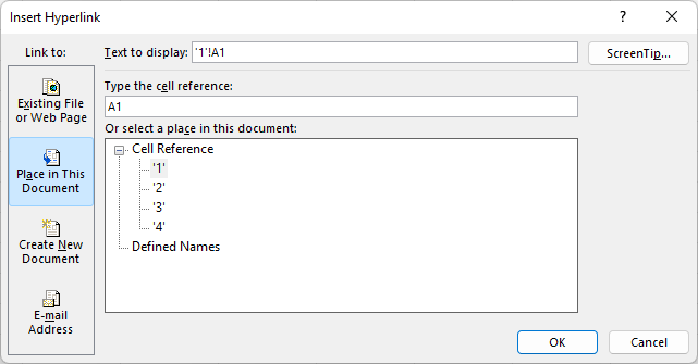
- Choose ‘Place in This Document’ from the left pane.
- Click on the desired sheet from the list, and optionally specify a cell reference.
- Confirm your selection by clicking ‘OK’.
How to link multiple cells at once in an Excel spreadsheet?
If you want to link multiple cells at once, you can use the HYPERLINK function:
- In a new cell, type =HYPERLINK(“cell_reference”, “link_text”).
- Replace ‘cell_reference’ with the target cell’s reference (e.g., A1) and ‘link_text’ with the desired display text.
- Drag the formula down and/or across to create hyperlinks for multiple cells.
What is the process for removing a hyperlink in Excel?
To remove a hyperlink in Excel, simply right-click the cell containing the hyperlink, and select ‘Remove Hyperlink’ from the context menu.
What shortcut can be used for inserting hyperlinks in Excel?
You can use the keyboard shortcut Ctrl + K to quickly open the ‘Insert Hyperlink’ dialog box in Excel.
How to link Excel sheets to a master sheet?
To link Excel sheets to a master sheet, follow these steps:
- Open the master sheet and the sheet(s) you want to link.
- Click on the cell in the master sheet where you want to insert the linked data.
- Type an equal sign (=).
- Switch to the sheet containing the data by clicking on its tab.
- Click on the cell with the data you want to link and press ‘Enter’.
- Repeat the process for other cells and sheets as needed.
How to create a hyperlink to an Excel file for email?
To create a hyperlink to an Excel file for email, follow these steps:
- Right-click the cell where you’d like to insert the hyperlink.
- Select ‘Insert Link’ from the context menu.
- Choose ‘Existing File or Web Page’ from the left pane.
- Navigate to the Excel file you want to link.
- Click ‘OK’ to confirm your selection.
The hyperlink can now be clicked in the email to open the linked Excel file.


