
When working with data in Excel, you’ll need to learn a collection of quick functions to get things done efficiently.
One key function is how to unhide columns that were previously hidden. It’s not hard, and there are numerous ways to do it.
To unhide columns in Excel:

- Click and drag to select the columns next to the hidden ones.
- Then, right-click on the selected area and choose “Unhide” from the menu.
- If you don’t see the “Unhide” option, it means there are no hidden columns nearby. After selecting “Unhide,” the hidden columns will instantly appear, and you can use and organize your data easily.
But that is only one way; check out the other methods to see which works best for you.

This article will discuss the various methods to unhide columns in Excel. By applying these techniques, you can work efficiently with your data, enhancing productivity and overall experience.
How to Identify Hidden Columns
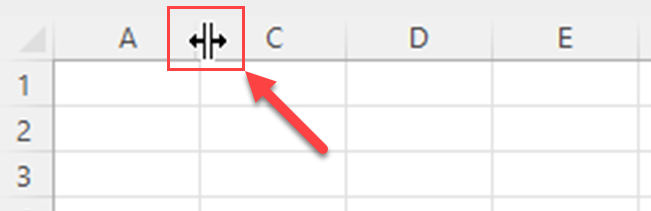
When columns are hidden in Excel, you can notice a double line or a gap between the visible column headers.
In the image below, you can see a double line between Column B and Column D. It says that the column between Column B and D is hidden.
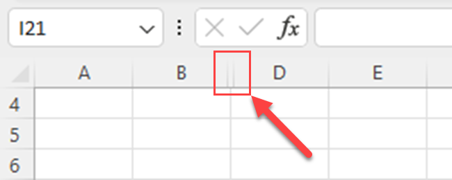
This is a visual cue that some columns are hidden, and you can interact with them if needed.
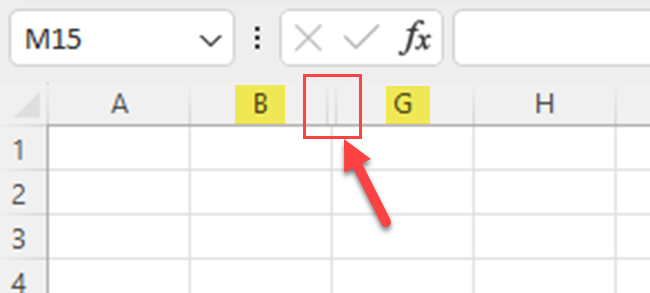
Another way to identify hidden columns is using the column letters. When you hide columns, you can’t see the column letter of the hidden column.

5 Ways to Unhide Columns in Excel
There are multiple ways to unhide columns in Excel. In this section, we will discuss 5 ways to unhide columns in Excel.
Each method will be followed by demonstrations to help you better understand the concepts.
Specifically, we will discuss the following methods:
- Unhide Columns Using the Context Menu
- Unhide Columns Using the Home Tab
- Unhide Columns Using the Keyboard Shortcuts
- Unhide Columns Using the Mouse Techniques
- Unhide Columns Using Excel VBA
1) How to Unhide Columns Using The Context Menu
When you want to reveal hidden columns in Excel, you can use the Context Menu.
You can follow the steps given below to unhide columns using the content menu:
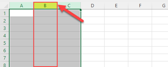
1) Select the adjacent columns of the hidden columns.
For example, if Column B is hidden, you have to select Columns A to C.
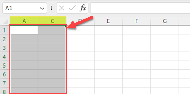
2) Right-click on the selected columns to open the context menu.
You can open it using the “Menu” key on your keyboard.
You can find the Menu key between the Right-side Alt key and the Right-side Ctrl key of your keyboard.
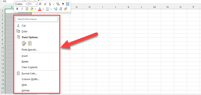
3) Choose Unhide from the context menu, and the hidden column(s) will become visible.
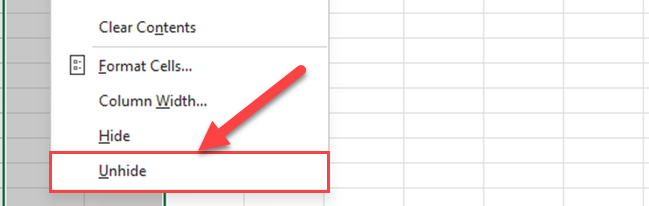
Then, Excel unhides the hidden columns. In this case, you’ll see the column B.
2) How to Unhide Columns Using The Home Tab
The Home tab in Excel is a powerful tool to manage and format your data efficiently. One handy feature available in this tab is the ability to easily unhide columns.
You can follow the below steps:
1) Firstly, select where the hidden columns are located.

To do this, click on the header of the column to the left of the hidden columns, then hold the Shift key on your keyboard, and click on the header of the column to the right of the hidden columns.
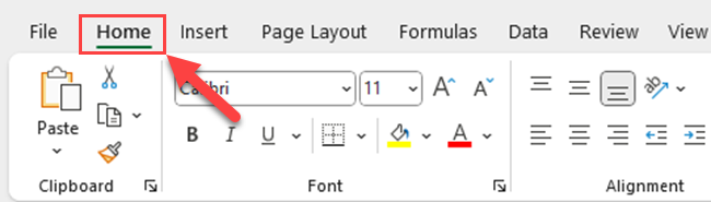
2) Go to the Home tab.
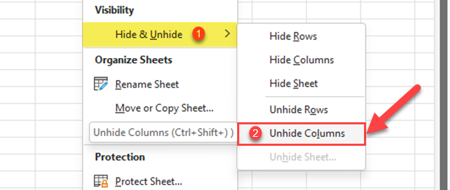
3) Go to the Cells group, and click on the Format option
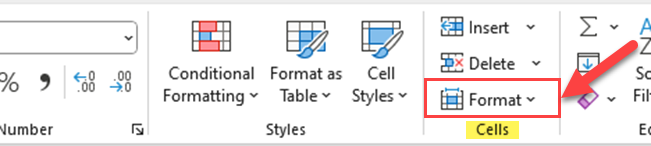
4) From the drop-down menu, choose Hide & Unhide and then select Unhide columns.

As soon as you click “Unhide Columns”, Excel will show the hidden columns.
3) How to Unhide Columns Using The Keyboard Shortcuts
There are several keyboard shortcuts that can help you unhide columns in Excel, making the process quick and efficient.
Here are a few useful ones:
- ALT + H + O + U + L: This key combination will unhide any hidden columns in Excel.
- ALT + O + C + U: This alternative keyboard shortcut performs the same function as the previous one.
- CTRL + SHIFT + 0: This shortcut unhides the hidden columns within the selected area of your worksheet. The last key of this shortcut is zero, not the uppercase letter “O”.
4) How to Unhide Columns Using The Mouse Technique
In addition to keyboard shortcuts, you can also use mouse techniques to unhide columns in Excel.
Follow the steps listed below to unhide columns using the mouse technique:
1) Locate the hidden column(s) by looking for a gap or double line between the visible column headers.
2) Hover your cursor to the right of the hidden column(s) until it changes into two parallel lines with two horizontal arrows.
3) Click and drag the double lines to the right to reveal the hidden column(s).
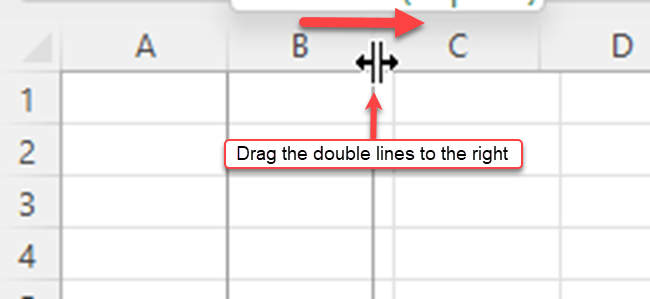
4) Release the mouse button when the column(s) are visible, and adjust the column width if necessary.
5) How to Unhide Columns Using Excel VBA
Excel VBA (Visual Basic for Applications) is a powerful feature that enables you to automate tasks and customize Excel operations.
To unhide a column that is hidden, we set the Hidden property to False:
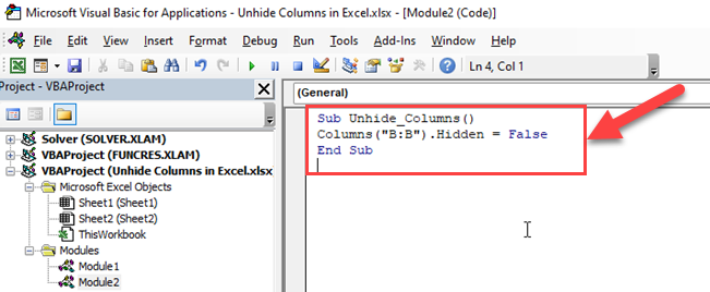
Sub Unhide_Columns()
Columns("B:B").Hidden = False
End Sub
This same method can be applied to unhide a range of columns:
Columns("B:D").Hidden = FalseYou can follow the below steps to apply the VBA code.
1) Press Alt + F11 to open the VBA Editor.
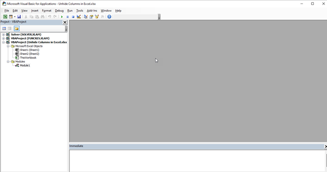
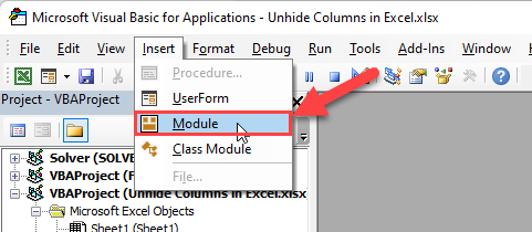
2) Click the “Insert” tab of the VBA Editor.
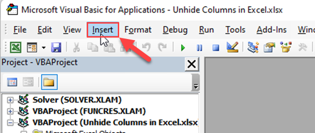
3) Select the “Module”.

4) Copy any of the above given VBA codes in the new module.
In short, with Excel VBA, you can easily control which columns are visible in your worksheets. This makes it simpler to handle your data, keeping it organized and easy to access.
How to Unhide Columns in Excel on MacOS
The process of unhiding columns and rows in Excel on Mac is relatively similar to Windows.

To unhide columns, select the columns on each side of the hidden column(s) by dragging through them. Then, right-click and choose “Unhide” in the shortcut menu or press ? + Shift + 0.
Just like on Windows, you can also use the ribbon to unhide columns on Mac:
- Click on the Home tab in the ribbon.
- In the Cells group, click on Format.
- Under Visibility, click on Hide & Unhide.
- Choose Unhide Columns.
By following these steps, you can easily unhide columns in Excel on MacOS.
How to Unhide All The Columns at Once?
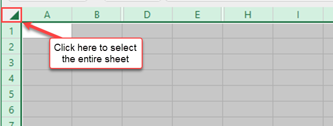
To unhide multiple columns, first select the entire worksheet by clicking on the green arrow in the left-top corner of the worksheet, or pressing Ctrl + A.
All cells of the worksheet will be selected.
Then, use any of the preferred methods to unhide columns. The reverse of this method also works when you want to hide multiple columns at once.
You can use either the Home tab, Cells group -Format option, or any other method to easily unhide columns at once. Any of these methods will unhide all the hidden columns.
How to Unhide the First Column in Excel?
To unhide the first column in Excel, you can use the following steps:
1) Type A1 in the Name Box and press Enter.
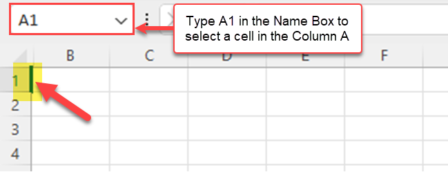
The A1 cell will now be selected, even if it’s hidden.
2) Go to the Home tab and click the “Format” option.

From the drop-down menu, choose Hide & Unhide and then select Unhide columns.
Then, Excel will unhide column A, and you can now view its content.
Learn more about DAX and Excel formulas by watching the following video:
Final Thoughts
As you learned, unhiding columns in Excel is easy and lets you show hidden columns in your sheets. Just choose nearby columns, right-click, and pick “Unhide” to make them visible again. You can also use any other method such as VBA to unhide columns in Excel.
Hiding columns is just as important as unhiding them. By learning to unhide columns, you’re not only decluttering your workspace, but you’re also revealing the full scope of your data, which aids in better analysis and decision-making.
Plus, it gives you more control over your data environment, allowing you to focus on what’s most relevant to you.
Frequently Asked Questions
In this section, you’ll find some frequently asked questions that you may have when unhiding columns in Excel.

How to reveal the first column in Excel
To unhide the first column in Excel, you can use the “Go To” option.
Press Ctrl + G to open the “Go To” dialog box, type A1 in the Reference field, and press Enter.
Once cell A1 is selected, right-click the header of any visible column and choose “Unhide” to reveal the first column.
What are the methods to display hidden rows in Excel
There are various methods to unhide hidden rows in Excel.
One approach includes selecting the rows above and below the hidden row, then right-clicking and selecting “Unhide” from the context menu.
Alternatively, you can use the “Format” command under the “Home” tab in the Excel ribbon, and click “Hide & Unhide” followed by “Unhide Rows.”
How to unhide rows using shortcuts in Excel
Unhiding rows in Excel with keyboard shortcuts can be faster and more convenient.
To unhide a row, first, select the row above and below the hidden row. Then press Alt + H + O + U + R to unhide the selected row.
For unhiding a column, you can press Alt + H + O + U + C after selecting the columns to the left and right of the hidden column.
How to unhide columns in Excel mobile
In Excel mobile, tap the selection arrow in the top-left corner, then drag to select the columns surrounding the hidden column.
After selecting the columns, tap the “Format” tab and choose “Hide & Unhide” followed by “Unhide Columns.”
This will reveal the hidden column on your mobile device.
How to uncover hidden sheets in Excel
To unhide a hidden sheet, right-click on any visible sheet tab, and select “Unhide” from the context menu.
This will open a dialog box listing hidden sheets in the workbook.
Choose the desired sheet and click “OK” to unhide it. Keep in mind that the hidden sheet might be protected, and you may need permission or a password to unhide it.


