
Welcome to the Exciting world of Excel formulas and functions!
At its core, lies the formidable duo: INDEX MATCH —a groundbreaking combination of functions that redefines data lookups and retrieval.
INDEX MATCH is a powerful formula that combines two Excel functions: the INDEX function and the MATCH function. The INDEX function returns a value from a specific position in a range, while the MATCH function returns the position of a value in a range. By using the MATCH function as arguments for the INDEX function, you can create a lookup formula that can return values from any table or range, regardless of the orientation, type, or size of the lookup value.

This article will be focused on INDEX MATCH, exploring its advantages over other lookup functions, offering a step-by-step guide to harnessing its power, and exploring some advanced applications for the avid Excel enthusiast.
So, whether you’re a seasoned data analyst or just learning Excel, read on to discover a tool that might just become your new spreadsheet sidekick.
Curious to unravel the mysteries of INDEX MATCH in Excel?
Let’s dive in by first taking a look at the Index and Match Functions.
Understanding the Index And Match Functions

To fully comprehend Index Match, it’s essential to dissect its core elements: the INDEX and MATCH functions. Each brings distinctive qualities, optimizing Excel’s data lookup capabilities when paired together.
Understanding the INDEX Function
The INDEX function in Excel acts as a map, guiding us to a specific cell within a particular range based on row and column numbers.

Let’s examine this more closely with an example:
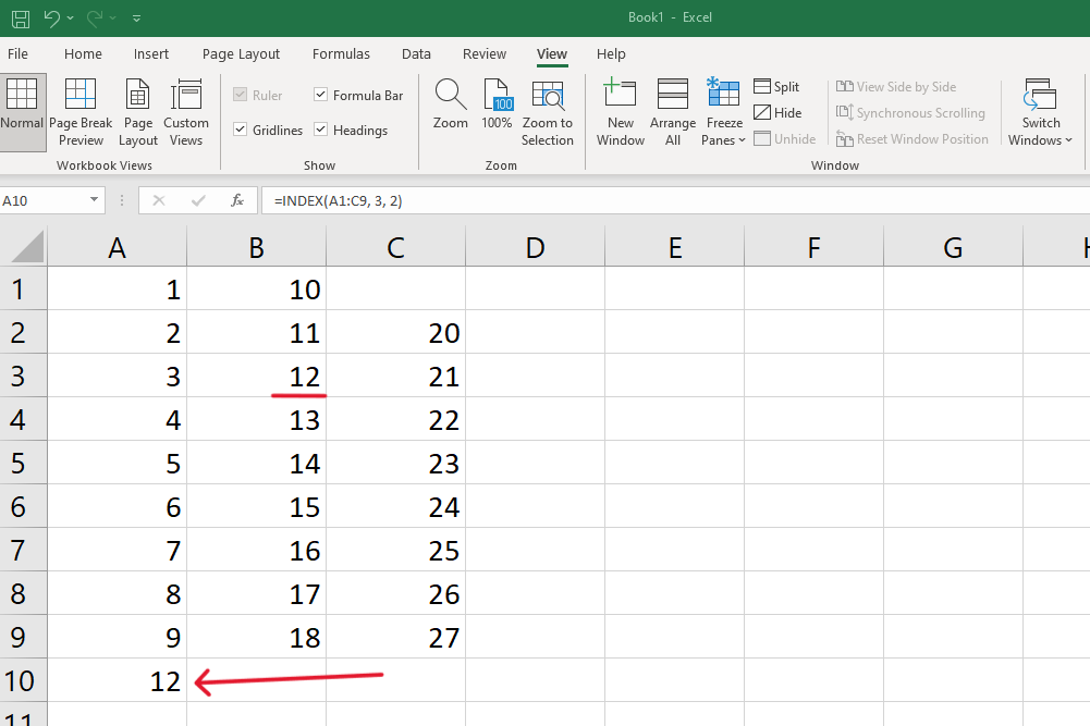
Imagine a range of cells (A1:C10). You want to find the value located at the intersection of the 3rd row and 2nd column within this range. Using the INDEX function like this: =INDEX(A1:C9, 3, 2) will lead you precisely to the value residing in cell B3.
Understanding the MATCH Function
The MATCH function operates like a search engine within Excel, scanning through a designated range for a specified item, and returning that item’s relative position. The function is formatted as “=MATCH(lookup_value, lookup_array, [match_type])“.
Here’s a simplistic breakdown:
- Lookup Value: It’s the specific item you’re searching for within a range.
- Lookup Array: It’s the range where Excel will look for the item.
- Match Type: How you want to search, allowing for exact or approximate matches.
That’s all it takes to construct the MATCH function. Next up, let’s take a look at the options available when running this formula, particularly when it comes to Match Type.
Match Type

This parameter is pivotal. It sets the tone for the search, determining if you want an exact match, or if you’re open to approximate matches. Here are the options:
0 (Exact Match): Excel will only return a position if it finds an exact match. If not, it returns an error. =MATCH(“Apple”, A1:A5, 0) – This will look for the exact word “Apple” in the range A1:A5.
1 (Less Than): Excel seeks the largest value that’s less than or equal to the lookup value. For this to work seamlessly, the lookup array should be in ascending order. =MATCH(5, {1,3,5,7,9}, 1) – If you’re searching for a value like 4, it will match with 3, the largest value less than 4.
-1 (Greater Than): Excel aims to find the smallest value that’s greater than or equal to the lookup value. Here, the lookup array must be in descending order. =MATCH(5, {9,7,5,3,1}, -1) – Searching for a value like 4 with this setup will match with 5, the smallest value greater than 4.
With its straightforward format and customizable parameters—lookup value, lookup array, and match type, the MATCH Function offers a tailored searching process, enhancing the ease and accuracy of data retrieval in Excel.
Match Function Example: Finding Product Code
Let’s say you have a column of product codes (A1:A11) and you want to find the position of a specific code, “PRD05”.
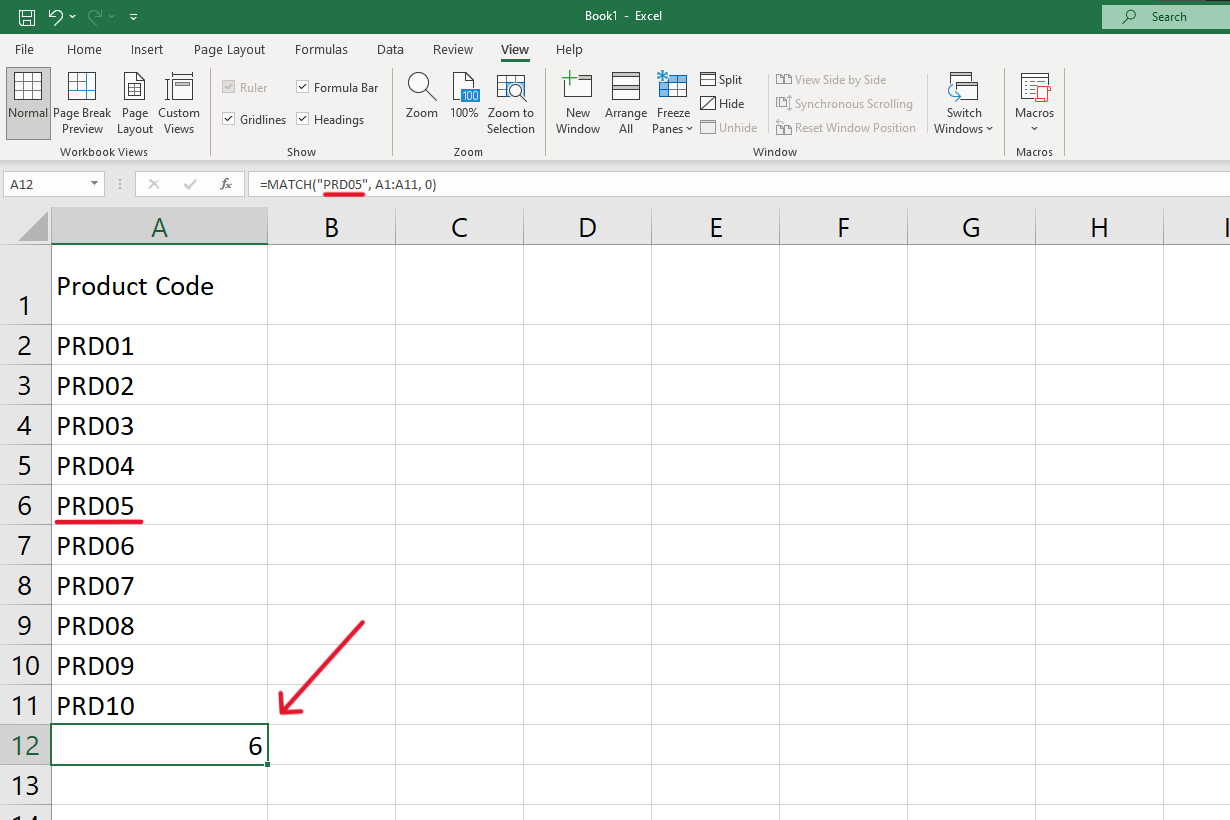
In a column filled with product codes (A1:A11), you want to find the position of a specific code, “PRD05”. Utilizing the MATCH function like this: =MATCH(“PRD05”, A1:A11, 0). The formula will probe the range and return the position where “PRD05” is found, considering it’s looking for an exact match due to the third argument being zero.
Combining INDEX and MATCH

In combination the INDEX and MATCH functions form an exceptional tool for executing advanced lookups. When utilized together they can extract data from a matrix with unmatched flexibility and accuracy, outperforming traditional lookup functions in efficiency and adaptability.
Why Combine INDEX and MATCH?
When united, the INDEX and MATCH functions amplify Excel’s lookup abilities. Combining INDEX and MATCH offers a versatile solution to find a lookup value within a table range, utilizing the row and column numbers.
Creating an INDEX MATCH formula involves integrating the MATCH function as an argument within the INDEX function. Here’s an example of how to craft the formula correctly:

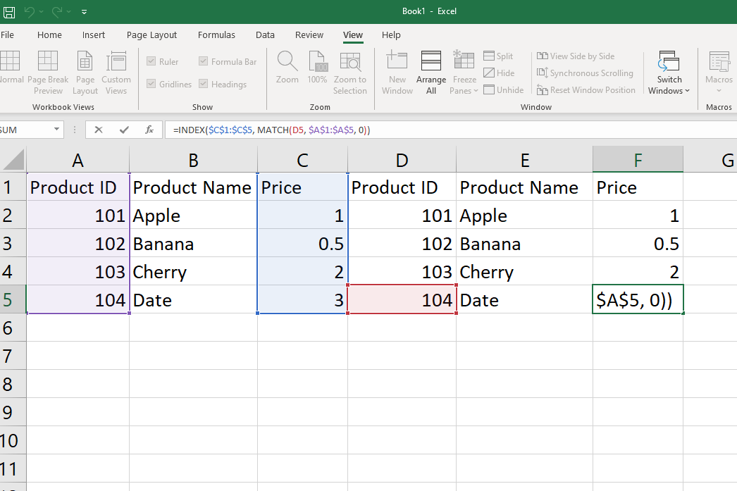
INDEX MATCH Example: Find the price of product in a table
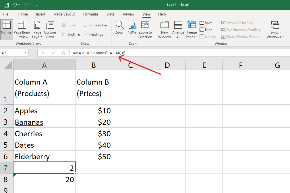
Suppose you want to find the price of a specific product in a table. You have product names in column A and their corresponding prices in column B.
Begin by using the MATCH function to find the row number of the product. =MATCH(“ProductName”, A2:A6, 0) This formula returns the row number where “ProductName” is located within the range.
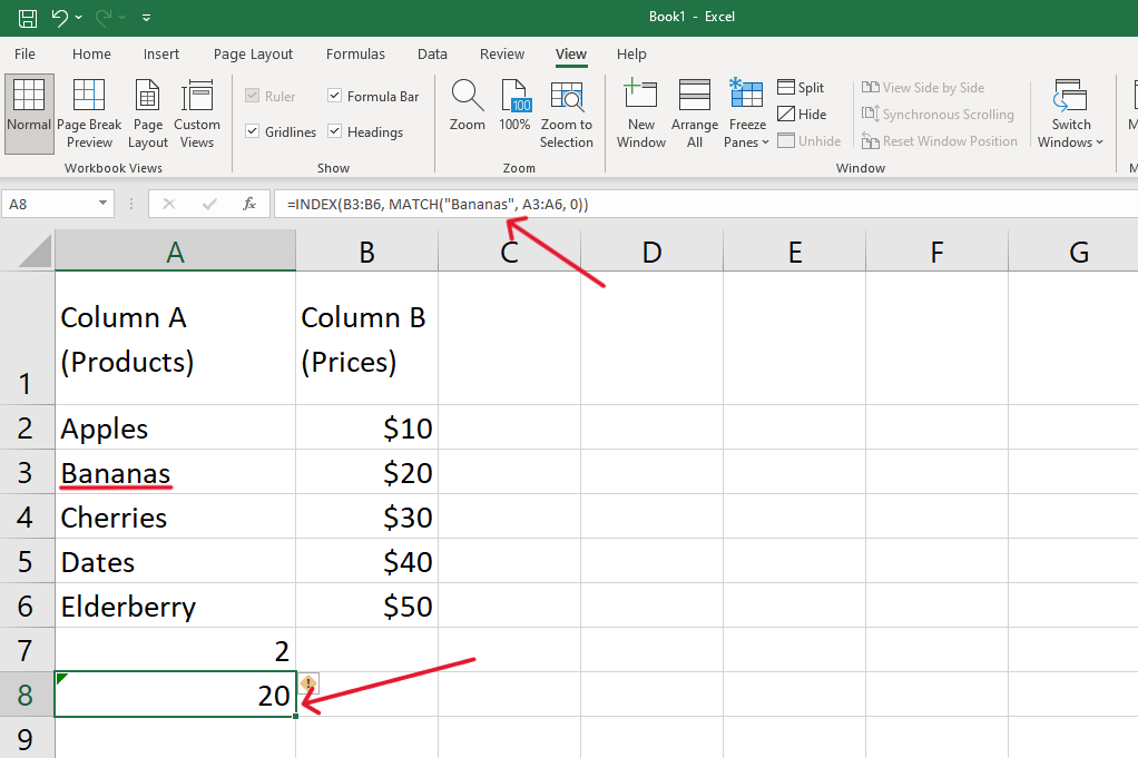
Now, you nest the MATCH function inside the INDEX function to find the price from column B. =INDEX(B2:B6, MATCH(“ProductName”, A2:A6, 0)) This combined formula precisely fetches the price of the specified product from the table.
The INDEX MATCH formula is versatile, allowing for the retrieval of values within the same column through relative referencing. It can also be expanded to incorporate a lookup table, ensuring accurate identification of the desired column position.
INDEX MATCH vs VLOOKUP Function
Both functions are used for lookup tasks, but INDEX MATCH holds certain advantages, like being able to perform lookups in any column or row, thus offering a more flexible “left lookup” and “right lookup” capability.
Now, let’s take a look at some of the other advantages it has over the VLOOKUP Function.
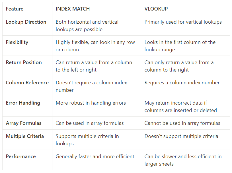
Why Choose INDEX MATCH Over VLOOKUP
Flexibility and Versatility: INDEX MATCH shows tremendous flexibility as it is not confined to looking up values in a table’s leftmost column, unlike VLOOKUP. This allows for a more dynamic lookup range, enabling the formula to return values from a column to the left of the lookup column.
Exact Match Precision: INDEX MATCH is precise in finding exact matches, thereby reducing the margin of error in the lookup. While VLOOKUP can also find exact matches, the former tends to execute this with more accuracy and consistency.
Two-Way Lookup: INDEX MATCH excels in performing two-way lookups. It can match both row and column numbers, navigating tables with ease, and extracting the correct data from intersections of rows and columns. This enhances its applicability in more complex lookup scenarios compared to VLOOKUP.
Handling Larger Datasets: When dealing with larger datasets, INDEX MATCH operates more efficiently. It computes and delivers results faster, ensuring that you can manage and analyze extensive data without experiencing significant slowdowns.
Advanced Lookups: INDEX MATCH can be integrated with other Excel functions, facilitating advanced lookups. It can be paired with functions like IF and ISERROR, allowing for more nuanced and conditional lookups that are beyond VLOOKUP’s native capabilities.
The precision offered by the INDEX MATCH combination in Excel marks it as an indispensable asset for comprehensive data analysis. While VLOOKUP remains a valuable tool, INDEX MATCH stands out due to its multifaceted capabilities. It offers flexibility in data directionality, intricate two-way lookups, and superior handling of large datasets, showcasing its superiority in various scenarios.
Another great alternative to VLOOKUP is HLOOKUP, you can ready more about it in our article here.
Common Scenarios for Using INDEX MATCH

The value of the INDEX MATCH combination becomes apparent when applied in various lookup scenarios.
Its flexibility allows users to execute lookups with enhanced precision and multi-dimensional criteria.
Let’s check out some use cases.
5 Great Use Cases for INDEX MATCH
- Lookup with Multiple Criteria: INDEX MATCH rises to the occasion when there are multiple criteria to consider in a lookup task. Unlike some functions that are limited to single-criterion lookups, INDEX MATCH can harmonize multiple conditions to fetch the most accurate data.
- Horizontal and Vertical Lookups: The function pair doesn’t shy away from any direction. Whether your lookup values are nestled in rows or columns, INDEX MATCH navigates through horizontal and vertical ranges with equal finesse, ensuring that no data point remains elusive.
- Left Lookup: Traditionally, certain lookup functions operate predominantly from left to right. However, INDEX MATCH rebels against this limitation, enabling users to perform left lookups with ease. This is crucial for instances where the lookup value is to the right of the return value.
- Handling Lookup Range in the Same Row or Column: INDEX MATCH also specializes in managing lookups within the same row or column. This is pivotal for cases where you want to maintain a consistent row or column reference, ensuring that the integrity of the data alignment is preserved.
- Two-Way Lookup: Embracing a bi-directional approach, INDEX MATCH facilitates two-way lookups, intersecting rows and columns, ensuring that you can pinpoint the exact location of your desired data in a matrix-style layout.
Through these varied applications, the value of the INDEX MATCH combination is vividly illustrated, substantiating its stature as an indispensable asset in data lookup and analysis.
Now, let’s check out some advanced techniques, these will come in useful on your Excel journey!
Advanced INDEX MATCH Techniques

Mastering these advanced Excel techniques unlocks a multitude of opportunities for enhanced data analysis and productivity.
Its compatibility with various functions and features ensures that it’s not just a lookup tool but a powerful formula constructor. Below are some the advanced techniques you can explore further:

Using INDEX MATCH across Multiple Worksheets
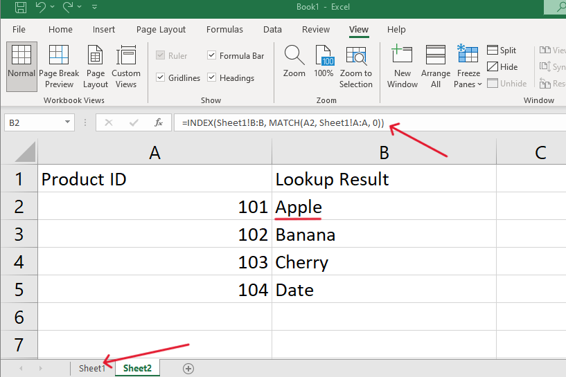
INDEX MATCH is not confined to operating within a single worksheet. It can transcend worksheet boundaries, allowing you to lookup values across multiple sheets. This cross-sheet operation ensures a comprehensive data search and retrieval, broadening the scope of your lookups.
Array Formulas with INDEX MATCH
INDEX MATCH also operates seamlessly with array formulas. This collaboration enables more complex calculations and lookups, facilitating the handling of multi-cell ranges and arrays, resulting in more nuanced and detailed data analysis and retrieval.
Combining INDEX MATCH with Other Functions
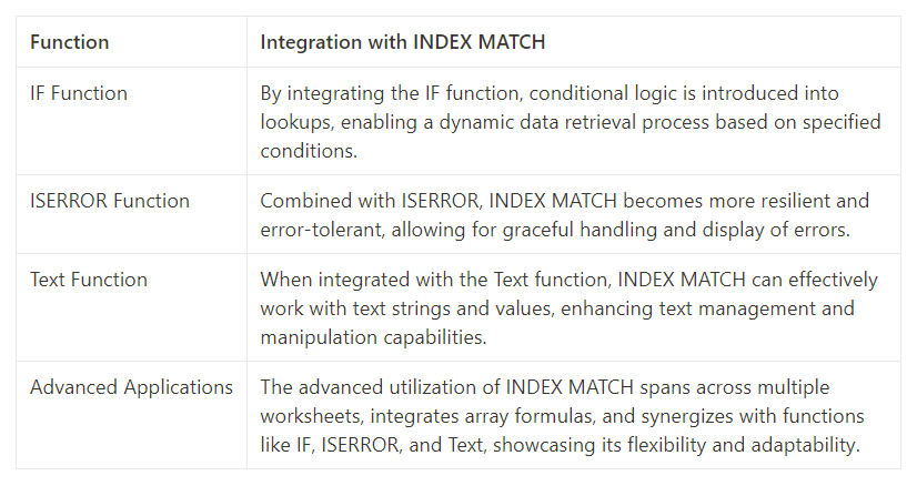
INDEX MATCH, in its advanced applications, is nothing short of a Swiss Army knife for Excel enthusiasts. Its compatibility with an array of functions and diverse use-cases certifies its status as an essential tool for sophisticated data lookups and analysis.
Troubleshooting Common Index Match Errors

INDEX MATCH in Excel sometimes leads to unexpected errors and roadblocks. These glitches can often be mystifying, disrupting the flow of data analysis and lookup operations. Let’s take a look at some practical solutions and troubleshooting tips to ensure your formulas work as intended.
Decoding Common Errors
Misalignment: A frequent misstep occurs when the lookup array and return array aren’t aligned. This misalignment can produce unreliable results. The key? Ensure that both arrays match in their row or column count.
Incorrect References: An easily overlooked error, it’s essential to cross-check that you’re pointing to the right row or column. A minor offset can drastically skew results.
Match Types Dilemma: Excel boasts multiple match types: exact match (0) and nearest match (-1 or 1). A common pitfall is selecting the wrong type, leading to unintended results.
Pro Tip: If you aim to pinpoint the exact price of a product, always opt for the exact match (0). Using a nearest match might fetch you a ballpark figure, but not the precise amount.
Navigating Empty or Missing Values
Empty strings or non-existent values can be silent disruptors in your lookup array, hindering the effectiveness of your INDEX MATCH formula.
Error Elegance: Employ the IFERROR() function for a graceful error handling approach. For example, if a value remains elusive, you can substitute an error with a friendly “Not Found” message.
Quick Fix: To seamlessly address missing values, leverage the formula =IFERROR(INDEX(…, MATCH(…)), “Not Found”).
Pristine Data Practice: Prior to delving into lookups, the best practice is to sanitize your data. Purging it of empty strings or phantom values ensures a smoother formula operation.
Best Practices and Tips

Improving your INDEX MATCH skills involves embracing best practices that enhance formula efficiency, flexibility, and reliability. Let’s explore some tips to improve your experience:
Syntax Confusion: Ensure that the syntax of INDEX MATCH is correct, referencing the return column first, then the lookup value and lookup column.
Indicating Match Type: Don’t forget to indicate the match type, ensuring accurate results.
Array Reference Size Mismatch: Ensure that reference arrays are of the same size for accurate results.
Lookup Value Absence: Confirm that the lookup value is present in the lookup array.
Reference Locking: Remember to lock references correctly while dragging the formula.
Static and Relative References: Ensure correct use of static and relative references in the formulas for accurate values or to avoid error messages.
Crafting Efficient Formulas: When working with INDEX MATCH, it’s essential to manage row and column numbers and cell references adeptly, ensuring that formulas are concise and readable.
Handling Variety in Lookup Columns: Versatility ensures that the formula remains functional and robust despite changes in the lookup range or array.
Maintaining and Updating Formulas: Maintaining the integrity of your formulas is pivotal. Regular updates and checks should be conducted to ensure that they remain accurate and responsive to the evolving data landscapes.
Embracing these best practices and tips will enhance your proficiency and effectiveness in leveraging the INDEX MATCH function in Excel for various lookup and reference needs.
Final Thoughts

The journey of learning Excel’s formulas and functionalities often leads us to powerful tools like the INDEX MATCH combo. As we’ve seen, this formula offers key advantages over traditional lookup methods. Its flexibility in handling cell references ensures precise data retrieval, regardless of the table orientation or size.
In our previous examples, we explored the INDEX function, seeing firsthand how it returns values from specified cell positions. With the MATCH function by its side, this combo elevates Excel lookups to new heights, offering closest match capabilities, even when dealing with the largest or smallest values in a range.
We also addressed the importance of understanding the first argument, second argument, third argument and the integral role they play in crafting these formulas. For those keen on diving deeper, exploring array formulas or even taking a glance at a video tutorial can offer more hands-on insights into how this formula works in diverse scenarios.
To fully grasp the power and efficiency of using INDEX MATCH, it’s essential to apply it practically. So let’s open a new instance of excel and get started putting the theory we have learnt to practice. Whether you aim to find a specific item’s index number or understand the formula’s mechanics, remember, this formula is pivotal for transforming data analysis and management in Excel.
Best of luck with your spreadsheets! May INDEX MATCH enhance your efficiency and become a reliable ally in your Excel usage.
Wanna learn more about Excel and modern data science tools, check out the Enterprise DNA YouTube channel.
Frequently Asked Questions
What exactly is the INDEX formula in Excel?
The INDEX formula in Excel acts as a guide, directing us to a specific cell within a designated range based on row and column numbers. The Excel INDEX function returns a value from a table range determined by these numbers.
How do the MATCH function and INDEX function differ?
While the Excel MATCH function is a detective tool that searches for a specific item in a range and returns its relative position, the Excel INDEX function retrieves a value from a particular position in a range or array.
Why would I use INDEX MATCH instead of VLOOKUP function in Excel?
The Excel INDEX MATCH is superior to VLOOKUP in many ways, offering flexibility in looking up values not just in the leftmost column but across any column. This capability ensures you can perform both “left lookup” and “right lookup” efficiently.
Is horizontal range lookup possible with INDEX MATCH?
Yes, INDEX MATCH can traverse both vertical and horizontal ranges. Whether your lookup values are in rows or columns, it navigates with precision, ensuring no data point remains hidden.
What do you mean by “left lookup”?
The term “left lookup” with INDEX MATCH signifies the function’s ability to return values from columns to the left of the lookup column, a capability often not present in functions like VLOOKUP.
If my data is in the same row, can INDEX MATCH handle it?
Yes, INDEX MATCH is adept at managing lookups within the same row, ensuring that the integrity of your data alignment remains intact.
What’s the significance of a two-way lookup in Excel?
A two-way lookup using the INDEX MATCH formula in Excel signifies the function’s ability to intersect both row and column numbers, helping users extract precise data from a matrix or table range.
How can I combine the Text function with INDEX MATCH?
Combining the INDEX MATCH formula with the Text function in Excel allows users to work effectively with text strings and values, providing enhanced text management capabilities.
How can I troubleshoot INDEX MATCH errors?
Some common errors can arise from things like empty string values, misalignment in the lookup array, or incorrect use of the match type. Proper formula auditing and understanding the source of these errors can aid in troubleshooting.
How can I optimize my use of INDEX MATCH?
Best practices for using INDEX MATCH include crafting efficient formulas, navigating through multiple criteria, handling a variety of lookup columns, and ensuring regular maintenance of your formulas.


