
Imagine Excel as your data superhero. It doesn’t just store numbers; it can make decisions for you! Enter the world of Logical Functions.
This is where Excel transforms into your trusted data detective. These functions are the key to making your spreadsheets work smarter, not harder.
Logical functions allow you to create powerful and efficient formulas by incorporating various conditions into your spreadsheet calculations. These functions are designed to work with logical values and test multiple conditions to return a specific result, such as TRUE or FALSE.

From the power of IF statements to the precision of the AND and OR functions, this article will explore how logical functions handle data and why they are your secret weapon for more efficient and accurate decision-making.
Mastering these functions is the key to turbocharging your spreadsheet skills.
Let’s unlock their power together!

Understanding Excel Logical Functions
Excel Logical Functions are like decision-making tools for your spreadsheets. These functions return logical values, either True or False, which you can use to perform various tasks in your spreadsheets.
They help Excel make choices for you based on certain conditions, making Excel a smart assistant that follows your instructions.
Here are a few basic logical functions to help you grasp it:

- IF: Returns a specified result based on whether a given condition is true or false.
- AND: Returns TRUE if all specified conditions are true; otherwise, it returns FALSE.
- OR: Returns TRUE if at least one of the specified conditions is true; otherwise, it returns FALSE.
- NOT: Returns the opposite logical value of a given expression.
- XOR: Returns TRUE if an odd number of the specified conditions are true; otherwise, it returns FALSE.

To get the most out of these functions, you can combine them to create more complex formulas.
For instance, you can use the IF function with AND, OR, or NOT functions to perform multiple tests and return specific results based on different conditions.
Remember that Excel’s logical functions only return True or False values, but you can use these values in other formulas or in conjunction with other functions to automate a wide range of tasks in your spreadsheets.
By mastering these Excel functions, you will become more efficient and confident in handling data and making decisions based on the results.
Basic Logical Functions in Excel
Microsoft Excel provides a set of commonly used logical functions that are the building blocks of decision-making in your spreadsheets. Let’s talk more about these functions and how you can make the most of them in Excel.
1. The IF Function

The IF function helps you compare something with what you expect and then act accordingly. It’s like saying, “If this is true, do that; otherwise, do something else.” So, when your condition is met(True), you get one result, and when it’s not met(False), you get a different result.
Syntax and Arguments
The syntax for the IF function is:
=IF(condition, value_if_true, value_if_false). It has three arguments:
- Condition: The condition you want to test, e.g. A1>70.
- Value_if_true: The value you want to return when the condition is true.
- Value_if_false: The value you want to return when the condition is false.
Examples:
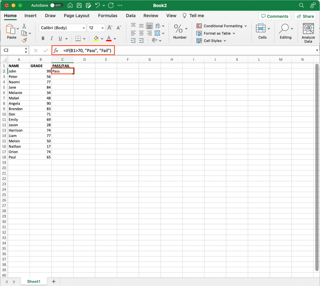
Suppose you have student scores in cell range B2, and you want to assign “Pass” or “Fail” based on a threshold score of 70. You can use an IF statement as follows:
=IF(B2>70, "Pass", "Fail")This IF formula tests whether the score in cell A1 is greater than 70. If it is, the logical value TRUE returns “Pass.” If not, it returns “Fail.”
If you want to get the Pass or Fail test results for the rest of students, simply drag down the fill handle to get the results for all students.

Note: Excel IF function is not case-sensitive. For instance, “=IF(A1=”apple”, “Yes”, “No”)” returns the same result as “=IF(A1=”Apple”, “Yes”, “No”)”
Handling Multiple Conditions

While the IF function can only handle one condition, you can nest multiple IF functions within each other to evaluate up to 255 conditions.
Example
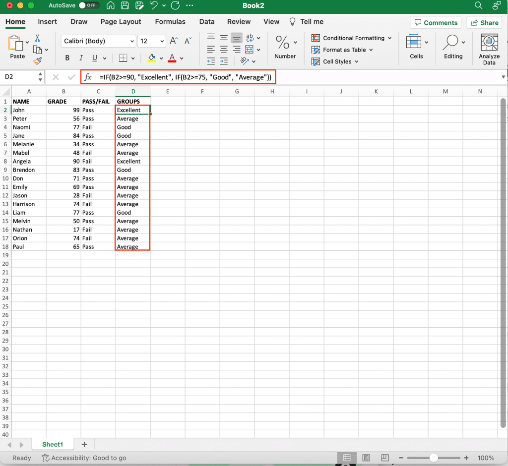
You want to categorize students based on their scores into three groups: Excellent, Good, and Average:
=IF(B2>=90, "Excellent", IF(B2>=75, "Good", "Average"))In this example, the first IF function checks if the score is 90 or above. If true, it returns “Excellent.” If false, it proceeds to the next IF function, which checks if the score is 75 or above. If true, it returns “Good,” and if false, it returns “Average.”

By using the IF function and its variations, you can enhance your Excel worksheets with more precise and adaptable calculations.
2. The AND Function

The AND function is used when you need to check if multiple conditions are met for a particular result. It follows the logic that “Both of these conditions must be true.” If all the conditions specified in the AND function are true, it returns TRUE; otherwise, it returns FALSE.
Syntax
The syntax for the AND function is as follows:
=AND(logical1, [logical2], ...)Here, logical1, logical2, etc., are the conditions you want to evaluate.
Example:
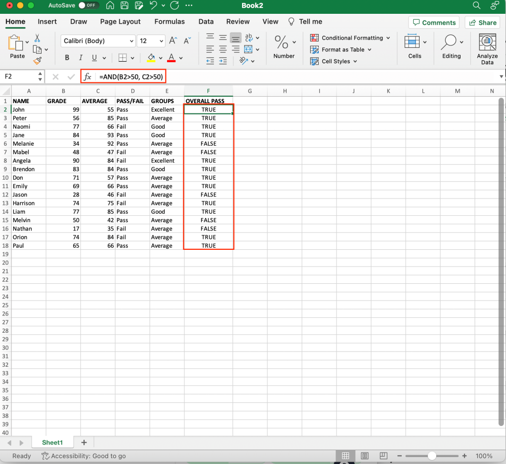
If you want to check whether the values in cells B2 and C2 are both greater than 50, you can use the following formula:
=AND(B2>50, C2>50)3. The OR Function

The OR function is the counterpart to the AND function. It’s used when you want to know if at least one of the specified conditions is true. It follows the logic that “At least one of these conditions must be true.” If any of the conditions are true, the OR function returns TRUE; otherwise, it returns FALSE.
Syntax
The syntax for the OR function is:
=OR(logical1, [logical2], ...)
Example:
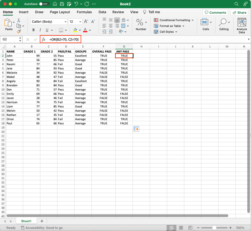
Let’s say you want to check if either cell B2 or C2 is greater than 70. You can use the following formula:
=OR(B2>70, C2>70)
By mastering the AND function in Excel, you’ll be able to evaluate multiple values, provide accurate results, and enhance your spreadsheet’s capabilities for processing complex data sets.
4. The NOT Function

The NOT function is a simple but powerful function that flips the truth value of a condition. If the condition is true, NOT makes it false, and vice versa. It’s like changing a yes to a no and a no to a yes. You can use it when you want to check if something is not the case, such as whether a task is not completed.
Syntax
The syntax for the NOT function is:
=NOT(logical)If you have a formula like =NOT(TRUE), the function will return FALSE. Likewise, if your input is =NOT(FALSE), the formula returns TRUE. You can also use cell references as logical arguments, such as =NOT(A1).
Example:
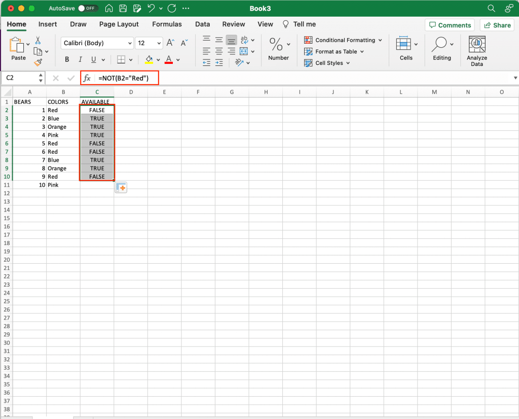
If you want to know what toys are available other than the ‘Red’ toy, you can use the formula
=NOT(B2="Red")All toys that are not red will return a result of TRUE while red toys will return the result of FALSE.
Excel’s NOT function offers valuable tool for evaluating and comparing logical expressions in your data. With this tool you can create powerful and dynamic formulas to solve various tasks in your spreadsheets.
5. The XOR Function

The XOR function is used when you want to check if an odd number of specified conditions are true. It follows the logic that “One and only one of these conditions must be true.” In other words, if an even number of conditions are true, XOR returns FALSE; if an odd number are true, XOR returns TRUE.
Syntax
The syntax for the XOR function is:
=XOR(logical1, [logical2], ...)Where logical1 is a required argument, and the subsequent arguments are optional. You can have up to 254 conditions as your arguments, which can be logical values, arrays, or references.
The XOR function returns TRUE only when there is an odd number of TRUE arguments. For example:
- =XOR(TRUE, FALSE) returns TRUE because there is one TRUE argument.
- =XOR(TRUE, TRUE) returns FALSE because there are two TRUE arguments, and both are not exclusive.
Example:
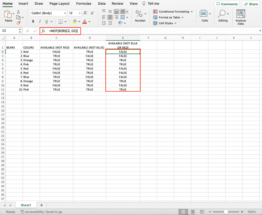
Here’s an example of how you can use the NOT and XOR functions together in a formula: Let’s say you have values in cells C2 and D2, and you want to check if both of them are TRUE or both of them are FALSE.

You can use the following formula:
=NOT(XOR(C2, D@))This formula will return TRUE if both values are the same (either both TRUE or both FALSE) and FALSE if they are different.
Now let’s talk about some additional and more advanced logical functions.
Advanced Logical Functions in Excel
Excel offers several advanced logical functions that allow users to create complex decision-making and data analysis formulas.
Here are some advanced logic functions in Excel.
1. IFS Function

The IFS function is a powerful decision-making tool introduced in newer versions of Excel. It allows you to evaluate multiple conditions and return different values based on the first true condition. The IFS function allows you to add up to 127 pairs of conditions and their corresponding results.
Instead of nesting multiple IF functions, you can simplify your formulas using IFS. It follows a straightforward logic: “If this is true, do this; if not, check the next condition.”
Syntax
The syntax for the IFS function is as follows:
=IFS(test1, value_if_true1, [test2, value_if_true2], ...)If any of the conditions are met, the function returns the corresponding result, and if none of the conditions pass, the function returns #N/A.
Example:
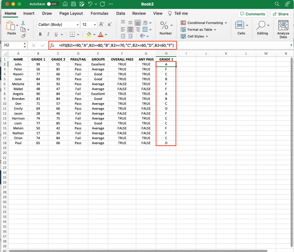
For example, you can use the IFS function to analyze a student’s grade:
=IFS(A1>=90,"A",A1>=80,"B",A1>=70,"C",A1>=60,"D",A1<60,"F")In this case, the IFS function checks the student’s score in cell B2 and returns the appropriate letter grade.
2. IFNA Function

The IFNA function is useful when your Excel formula might return a #N/A error. This function allows you to display a custom message or value when the formula yields a #N/A error.
Syntax
The syntax for the IFNA function is:
=IFNA(value, value_if_na)If the value is not #N/A, the function returns the value, and if it is #N/A, the function returns the specified value_if_na.
Example:
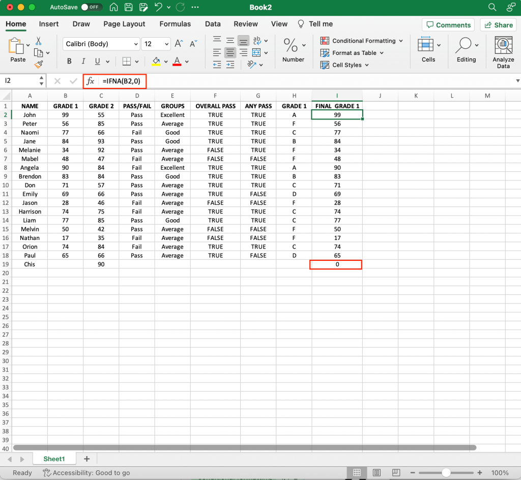
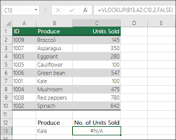
If you want to replace a #N/A value with a zero when a students grade is missing, use this:
=IFNA(B2,0)If the IFNA function fails to find a value in the range B1, the IFNA function will return “0” instead of the #N/A error as seen in I19.
3. IFERROR Function

Similar to IFNA, the IFERROR function is designed to handle errors in your formulas. However, IFERROR covers all types of errors, not just #N/A errors.
Syntax
The syntax for the IFERROR function is:
=IFERROR(value, value_if_error)If the value does not generate an error, the function returns the value; otherwise, it returns the specified value_if_error.
Example:
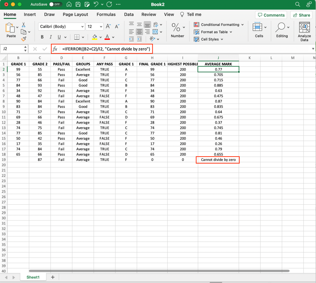
An example of IFERROR usage is:
=IFERROR((B2+C2)/I2, "Cannot divide by zero")In this case, if cell I2 is equal to zero, Excel would return a #DIV/0! error, but IFERROR will display “Cannot divide by zero” instead.
4. SWITCH Function

The SWITCH function allows you to choose a value from a list by comparing it with a specified expression.
Syntax
The syntax for the SWITCH function is:
=SWITCH(expression, value1, result1, [value2, result2],..., [default])If the expression matches any of the values, the function returns the corresponding result; if not, it returns the optional default value or #N/A if the default value is not provided.
Example:
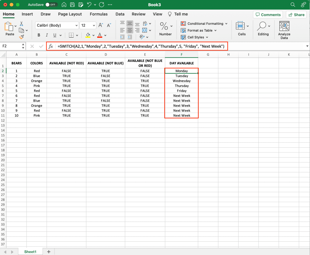
You can use the SWITCH function to return a category for numerical ratings:
=SWITCH(A2,1,"Monday",2,"Tuesday",3,"Wednesday",4,"Thursday",5, "Friday", "Next Week")This formula checks the value in cell A2 and returns the corresponding category, or “Next Week” if the value does not match any of the listed options.
There are more logical functions that we haven’t mentioned but rest assured that by mastering the listed functions, you will be well on your way to logical function mastery.
Encountering Errors in Logical Functions
While logical functions in Excel are powerful tools for decision-making and data analysis, they can also produce errors under certain circumstances. Understanding these errors and how to handle them is crucial to working effectively with these functions.
Here’s an overview of the common errors you might encounter:
1. #VALUE! Error
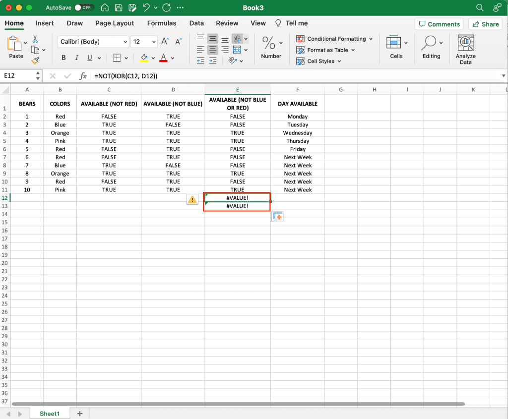
The #VALUE! error occurs when Excel can’t understand one or more of the values or arguments in your logical function. This could be due to various reasons, such as incompatible data types or improper syntax.
Example: You use the IF function with a text value in the logical_test argument instead of a logical test, like this:
=IF("Apples", "Good", "Bad")To fix this error, make sure the logical_test argument contains a valid logical expression.
2. #DIV/0! Error
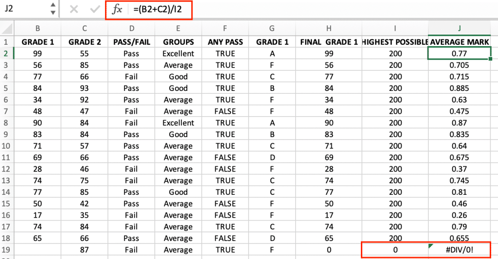
The #DIV/0! error occurs when you attempt to divide a number by zero. Logical functions can often involve mathematical operations, and if a division operation results in zero as the divisor, this error will occur.
Example: You use the IF function to calculate the average score, but one of the scores is zero:
=IF(A1=0, "Invalid", SUM(B1:B3) / A1)To avoid this error, ensure that you don’t divide by zero by using appropriate conditions or error-handling mechanisms.
3. #NAME? Error
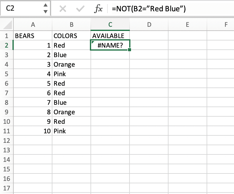
The #NAME? error happens when Excel doesn’t recognize a function or an argument within a function. This is typically due to a misspelled function name or an unrecognized argument.
Example: You attempt to use a logical function called “IFFUNC” instead of the correct “IF” function:
=IFFUNC(A1=1, "Yes", "No")To resolve this error, double-check the function name and argument structure to ensure accuracy.
4. #N/A Error
The #N/A error stands for “Not Available” and is often returned when a lookup function fails to find a specified value in a given range.
Example: You use the IF function to search for a value in a range, but the value is not present:
=IF(ISNA(MATCH("X", A1:A5, 0)), "Not Found", "Found")To handle this error, you can use the ISNA function to check if the result of the MATCH function is #N/A and then provide an alternative result.
5. Handling Errors

Excel offers functions like IFERROR, ISERROR, and ISERR to help you manage errors in logical functions. These functions allow you to define what should be displayed or calculated when an error occurs, making your spreadsheets more robust and user-friendly.
Understanding these common errors and how to address them ensures that your functions work as intended and that your Excel worksheets remain error-free and reliable for decision-making and data analysis.
Final Thoughts

In this article, you’ve unlocked the power of logical functions in Excel.
Now, you can confidently analyze and make data-driven decisions using functions like IF, AND, OR, XOR, and NOT, which compare values and generate TRUE or FALSE results.
Make your spreadsheets efficient, organized, and error-free by using these functions effectively. When working with arrays or multiple cells, remember to use absolute or relative references to maintain data flow.
With this strong foundation, keep exploring and practicing these functions in your daily tasks. You’ll soon become an expert Excel user. Happy spreadsheet-ing!
As you continue to master Excel explore tips and tricks to master and integrate additional powerful tools like Power BI and Python:
Frequently Asked Questions
How can I combine multiple conditions in Excel?
You can combine multiple conditions in Excel by using the AND, OR, and NOT functions within a single formula. This can be particularly useful for more complex decision-making in your spreadsheets. For example, you may use the following formula to test if a value in cell A1 is both greater than 10 and less than 20:
=AND(A1>10, A1<20)
What are the benefits of using a logical function?
Using logic functions can help you:
- Automate decision-making and actions based on cell values.
- Simplify complex formulas by breaking them down into smaller, logical components.
- Improve the accuracy and consistency of your spreadsheet by reducing manual data entry and error.
- Create more dynamic and responsive spreadsheets that adapt based on variable data.
How are logical functions used with other types of functions?
These functions can be combined with other types of functions for more sophisticated data analysis and decision-making. This may involve using logical functions within text, mathematical, statistical, or lookup functions, for example.
One common use case is conditional formatting, where you can apply different formatting rules based on specific criteria using the IF function.
What are the main operators used in a logical function?
The main operators used in logical functions include:
- Equal to (=): Compares if two values are equal.
- Less than (<): Compares if one value is smaller than another.
- Greater than (>): Compares if one value is bigger than another.
- Not equal to (<>): Compares if two values are not equal.
- Less than or equal to (<=): Compares if one value is smaller than or equal to another.
- Greater than or equal to (>=): Compares if one value is bigger than or equal to another.
These operators play a key role in defining the conditions used within these functions in Excel.


