HLOOKUP in Excel: What Is It & How To Use It

HLOOKUP function is an extremely useful tool in Excel. It helps you find and get data from a table that’s arranged horizontally.

Think of the “H” as standing for “horizontal”.

The main job of HLOOKUP is to find what you’re looking for and give you the related information from a specific row in that table. This is handy when you have big piles of data because it looks for matches in rows instead of columns.

The HLOOKUP function syntax is as follows:

=HLOOKUP(lookup_value, table_array, row_index_num, [range_lookup])

• lookup_value: This is the value you want to search for in the first row of the table.
• table_array: This is the range of cells that make up the table in which you want to search.
• row_index_num: This is the row in the table from which you want to retrieve the corresponding value.
• [range_lookup]: This is an optional argument, either set to TRUE or FALSE. When set to TRUE, the function will perform an approximate match, and when set to FALSE, it will perform an exact match.

Even though there’s a fancier function called XLOOKUP in newer Excel versions, HLOOKUP is still important. That’s because XLOOKUP only works in the latest Excel versions like Microsoft 365, Excel 2021, and Excel for the web.

So if you’re not using those, HLOOKUP is a must-learn tool in Excel.

Let’s get started!

Understanding HLOOKUP

HLOOKUP, or Horizontal Lookup, is a powerful function in Excel that helps you find corresponding data in a table by searching a row for matching data and outputting the value from a specified column. It works similarly to the VLOOKUP function, which searches for values in a column rather than a row.

To use HLOOKUP in Excel, first, you need to understand the syntax of the function.

The Syntax of Hlookup

Using the HLOOKUP function in Excel allows you to perform horizontal lookups by searching for a value in the first row of a table and returning the corresponding value from a specified row in the same table. The syntax for the HLOOKUP function consists of four arguments:

=HLOOKUP(lookup_value, table_array, row_index_num, [range_lookup])

• lookup_value: This is the value you want to search for in the first row of your table. It can be a cell reference, a numeric value, or a text string.
  A text string is a series of characters enclosed in double quotes such as “marks”, while a number can simply be typed in directly, like 100.
  A cell reference, on the other hand, is the reference to a cell in the worksheet, like B3 or C5.
• table_array: This is the range of cells representing the table where you want to perform the lookup. Be sure to include all relevant rows and columns.
• row_index_num: This is the row number in your table from which you want to retrieve the corresponding data. The row_index_num must be a positive integer.
• range_lookup: This is an optional argument, represented by a Boolean value. It can take two values:
  • TRUE (default): Returns an approximate match, where the value in the first row must be equal to or less than the lookup_value.
  • FALSE: Searches for an exact match, where the value in the first row must be exactly equal to the lookup_value. If an exact match isn’t found, the function will return an error.

In the next section, we’ll look at some HLOOKUP examples.

Using HLOOKUP in Excel

Example

The table below shows the marks of students in mathematics and science.

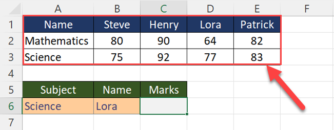
Suppose you want to find Lora’s marks for the Science subject.

Then, you can use the following formula.

=HLOOKUP(B6,$B$1:$E$3,3,FALSE)

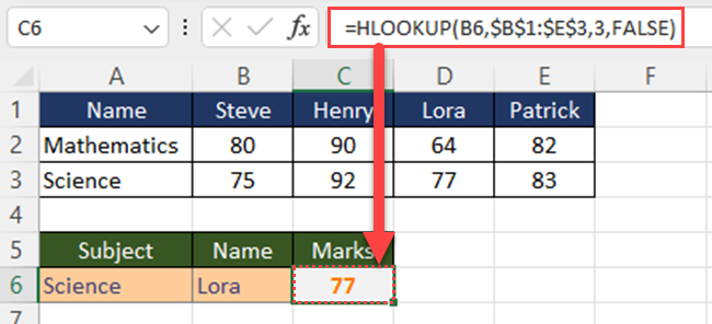
In this formula, B6 is the lookup value (You can even type “Lora” within quotes), $B$1:$E$3 is the table array, 3 is the row index number, and FALSE indicates an exact match.

Excel will scan the top row, locate “Lora,” and then the HLOOKUP function returns the corresponding value from row 3.

You get the matching value of 77, as expected.

Here are some additional tips to help you make the most of Excel’s HLOOKUP function:

• If the lookup value is a text, enclose it in double quotes.
• The table_array can include any number of columns and rows. But make sure that the top row contains the search value. In the top row, you can put text, numbers, or even logical values like “true” or “false.”
• If you change the position of the original data, ensure to adjust the table_array accordingly.
• If the search for an exact match returns an error, verify that the spelling and formatting of the lookup_value match the content in the first row.

Now you have the knowledge to confidently use the HLOOKUP function in Excel. With practice, you will find it to be an indispensable tool for retrieving information from horizontal tables in your worksheets and workbooks.

Dealing with HLOOKUP Errors

Errors in Microsoft Excel can be frustrating, especially when using HLOOKUP.

In this section, we will focus on some common HLOOKUP errors, such as #N/A, #VALUE!, and #REF!, and how to resolve them.

#N/A Error

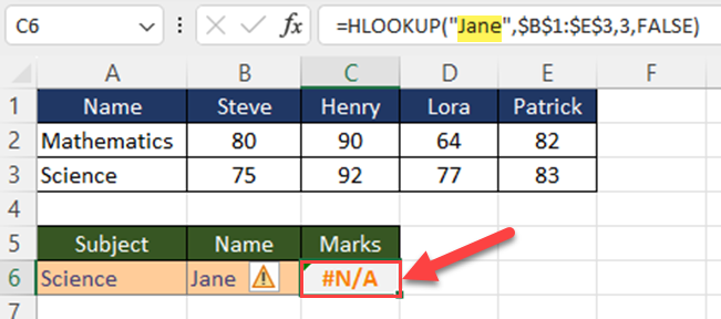
This error occurs when HLOOKUP cannot find the specified lookup value in the first row of the table or range.

To fix this:

1. Double-check if the lookup value you entered is correct and present in the first row of the table or range.
   In the above example, the name “Jane” is not in row number 1. So, the HLOOKUP function returns #N/A.
2. Make sure your lookup value is in the correct format (e.g., text, number, date). Sometimes, they appear similar but have different formats.
3. If you’re using an approximate match (range_lookup set to TRUE), ensure that the data in the first row of the table or range is sorted in ascending order.

#VALUE! Error

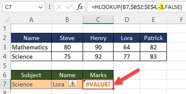
This error occurs when the row_index_num parameter in the HLOOKUP function is less than 1.

To fix this:

1. Ensure that your row_index_num is a positive integer that corresponds to the row number from which you want to retrieve the value.
2. Verify that any cell references or formulas used to determine the row_index_num produce a valid result.

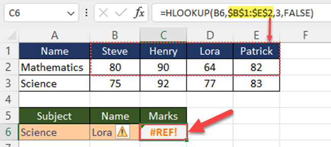
#REF! Error

This error occurs when the row_index_num parameter is greater than the number of rows in the table_array.

To fix this:

1. Review the row_index_num parameter and make sure it doesn’t exceed the number of rows present in the table_array.
2. Double-check if your table_array reference is correct and includes all the necessary rows.
   In the above image, the HLOOKUP formula doesn’t include row number 3. So, the formula returns #Ref! error.

Remember that handling errors in HLOOKUP is essential to ensure the accuracy and reliability of your Excel calculations.

By understanding the causes of these errors and applying the suggested solutions, you will be better equipped to work through any HLOOKUP-related challenges that may arise.

So, proceed with confidence and keep refining your HLOOKUP skills.

Using HLOOKUP with Exact and Approximate Matches

When using HLOOKUP, you have the option to search for an exact match or an approximate match, depending on the value of the range_lookup argument.

Read on as we look at both options and learn how to use them effectively.

Exact Match

To look for an exact match, set the range_lookup argument to FALSE.

This will tell Excel to find an exact match for the lookup_value in the first row of the table_array.

If an exact match is not found, the HLOOKUP function will return an error.

For example:

=HLOOKUP("Henry",$B$1:$E$3,3,FALSE)

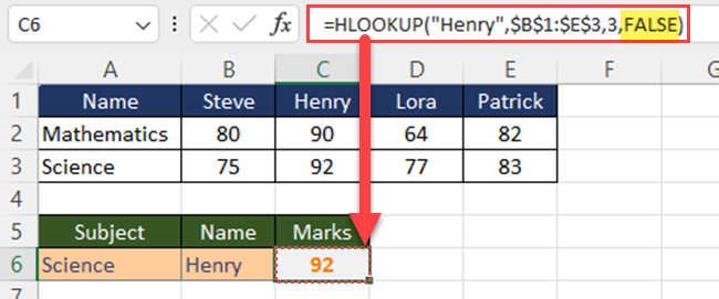
In this example, you are searching for an exact match of the name “Henry” within the range B1 to E3. Since the function matches the exact value, you’ll get 92 for the result.

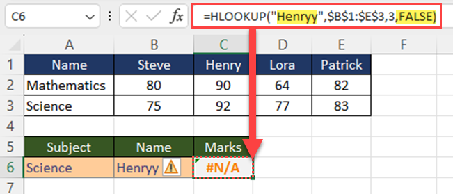
If you change the lookup value to “Henryy”, you’ll get an error value. The rea

Approximate Match

If you are looking for an approximate match instead, set the range_lookup argument to TRUE or leave it empty.

This option is useful when you want the HLOOKUP function to return the next largest value less than the lookup_value in case an exact match is not found.

Keep in mind that you have to sort the table in ascending order for this option to work properly.

Example

The below table shows the discount percentages for minimum quantities

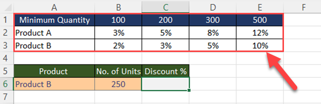
Suppose you want to find the applicable discount for the given quantity of the selected product.

In this situation, you can’t use the exact match function that we discussed earlier. You have to use the HLOOKUP function with the approximate match.

Then, you can use the following formula.

=HLOOKUP(B6,$B$1:$E$3,3,TRUE)

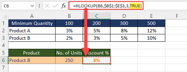
In this example, you provide the same range and lookup_value as before but specify TRUE for the range_lookup argument.

If an exact match is not found, the function will return the closest value less than the lookup_value in the specified row.

In conclusion, the HLOOKUP function in Excel is a versatile tool for finding exact and approximate matches within a horizontal dataset.

By using the range_lookup argument effectively and adjusting it to either TRUE or FALSE, you can optimize your search process and return the desired values efficiently.

Advanced Uses of HLOOKUP

In this section, we’ll explore advanced uses of the HLOOKUP function in Excel, utilizing various elements like row_index, table array, range_lookup, and more.

Handling Wildcard Characters

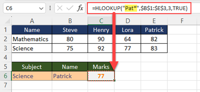
HLOOKUP can work with wildcard characters like ‘?’ and ‘*‘. The ‘?‘ matches any single character, while ‘*’ matches any sequence of characters.

For example, if your lookup value is “Pat*”, HLOOKUP will search for any value in the topmost row that starts with “Pat”.

Working with External References and Named Ranges

You can use HLOOKUP to retrieve data from another workbook or named range. To do this, specify the table_array parameter as an external reference or named range.

For example, =’C:\Folder[Workbook.xlsx]Sheet1′!A1, where the file path and sheet name are defined for an external reference, or ‘NamedRange’ for a named range.

Using Array Formulas

HLOOKUP can be used with an array formula to work with multiple values.

For example, if you want to get results from multiple rows, you can include all row numbers as a constant (enter row numbers with ‘{‘ and ‘}’ ) in a single HLOOKUP function.

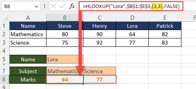
This way you can save valuable time.

Always ensure your HLOOKUP function uses the appropriate row_index, table_array, and range_lookup parameters for accurate results.

By mastering these advanced techniques, you can take full advantage of Excel’s powerful HLOOKUP function.

Differences between HLOOKUP and VLOOKUP

HLOOKUP and VLOOKUP are both useful Excel functions for searching and retrieving data in a spreadsheet.

However, there are several differences between them that you need to understand to use them effectively.

This section will help you grasp these key distinctions and understand when to use each function appropriately.

HLOOKUP stands for Horizontal Lookup, which means it searches for a value horizontally across the rows in a table. To use HLOOKUP, your data needs to be organized in rows, with the lookup value appearing in the top row of the table.

On the other hand, VLOOKUP stands for Vertical Lookup, and as the name suggests, it looks for a value vertically down the columns in a table.

Another significant difference is the way HLOOKUP and VLOOKUP handle the row or column index for returning data. VLOOKUP uses a column index, while HLOOKUP uses a row index.

By understanding these differences between HLOOKUP and VLOOKUP, you can confidently choose the right function for your particular data organization and effectively retrieve the information you need in Excel.

Final Thoughts

Remember, to obtain accurate results from the HLOOKUP function, make sure the data table is organized horizontally with the search values in the first row. As you become more comfortable with using HLOOKUP, you may find this function invaluable in retrieving information across different levels of your data.

In summary, working with HLOOKUP is efficient and convenient across various versions of Excel.

By understanding its formula syntax and applying it to your data, you can effectively retrieve and analyze important information in your spreadsheets. However, if you are a Microsoft Excel 365 user, consider using the XLOOKUP.

If you are interested in learning how to create a simple Lookup Table from subtotal rows in Power BI, watch the below video.

Frequently Asked Questions

How does the HLOOKUP function work in Excel?

HLOOKUP (Horizontal Lookup) function in Excel searches for a specified value in the topmost row of a table and returns a corresponding value from any specified row in the same column.

The function has four arguments: lookup_value (value to find), table_array (table where data is looked up), row_index_num (row number to return a value from), and range_lookup (optional, for approximate or exact match).

What are the steps to apply HLOOKUP in Excel?

To apply HLOOKUP in Excel, follow these steps:

1. Click on the cell where you want the result.
2. Type the formula =HLOOKUP(lookup_value, table_array, row_index_num, [range_lookup]).
3. Fill in the arguments: lookup_value, table_array, row_index_num, and [range_lookup].
4. Press Enter. The HLOOKUP function will return the corresponding value from the specified row.

Can HLOOKUP be combined with IF condition?

Yes, HLOOKUP can be combined with an IF condition. You can use the IF function to perform conditional operations based on the outcome of the HLOOKUP function.

For example: =IF(HLOOKUP(lookup_value, table_array, row_index_num, FALSE)=desired_value, “Result if true”, “Result if false”).

How to use HLOOKUP with multiple lookup values?

To use HLOOKUP with multiple lookup values, you can either nest multiple HLOOKUP functions using commas or use an array formula.

Alternatively, consider using other functions like XLOOKUP, INDEX and MATCH combined, which can handle numerous lookup criteria more efficiently.

How does HLOOKUP differ from VLOOKUP?

The main difference between HLOOKUP and VLOOKUP is the orientation of the lookup.

HLOOKUP searches horizontally (across rows) while VLOOKUP searches vertically (down columns).

HLOOKUP looks for values in the first row of a table and returns a value from the same column in a specified row, whereas VLOOKUP searches in the first column of a table and returns a value from the same row in a specified column.

Are there any alternative functions to HLOOKUP, such as XLOOKUP?

Yes, there are alternative functions to HLOOKUP. One of them is XLOOKUP, introduced in Excel versions starting from Office 365.

XLOOKUP is more flexible and powerful than HLOOKUP, as it allows you to search both horizontally and vertically, handles arrays, and provides additional options like if_not_found and match_mode.

Another alternative is the combination of INDEX and MATCH functions, which can perform complex lookups and handle multiple criteria efficiently.