
So you’ve cruised through the basics, tackled the intermediate stuff, and now you’re ready to wrestle with the big guns — Excel’s advanced formulas! Excel has many advanced functions and formulas for sophisticated calculations, so it’s useful to have a guide that pinpoints the ones you need.
This Excel formulas cheat sheet covers advanced forecasting formulas, statistical analysis, data manipulation functions, error handling, and more.
This reference will equip you with the knowledge of how to use these advanced functions. Each formula is accompanied by clear explanations, syntax, and practical examples to help intermediate Excel users become advanced power users.

Please downloaded and print out the cheat sheet and keep it handy.
Ok, let’s get started.
Firstly, let’s get into Array formulas.
Array Formulas
Our beginner cheat sheet shows you how to sort and filter your data manually. Advanced users do this programmatically with array formulas.
Array formulas allow you to perform calculations on multiple cells simultaneously. These are three key functions:
UNIQUE
SORT
FILTER
Some of these functions are only available in the most recent versions of Microsoft Excel.
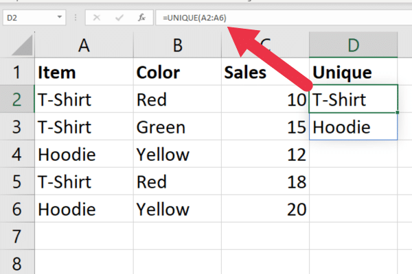
1. UNIQUE Function
The UNIQUE function accepts a range and returns a list of unique values.

Suppose you have sales data for clothing items. To find the unique items in column A, use this formula:
=UNIQUE(A2:A6)
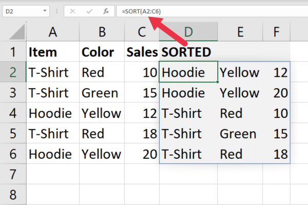
2. SORT Function
The SORT function sorts the contents of a range. The syntax is:
SORT(array, [sort_index], [sort_order], [by_col])
array: the range of values to sort.
sort_index: the column to sort (1 by default)
sort_order: 1 for ascending (default) or 2 for descending).
by_col: TRUE to sort by column (default) or FALSE to sort by row.
The last three arguments are optional, and the defaults are usually what you want.
To sort the sample data by the first column, use this formula:
=SORT(A2:C6)
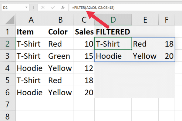
3. FILTER Function
The FILTER function lets you filter a range on a specific condition. This is the syntax:
=FILTER(array, include, [if_empty])
array: the range to filter.
include: the condition that determines which values to filter.
if_empty: specifies what to return if no values meet the filtering criteria (default is “”).
Suppose you want to filter the rows in the sample data to only show where the sales value is greater than $15. Use this formula:
=FILTER(A2:C6, C2:C6>15)
Randomizing Excel Functions
Our intermediate cheat shows how to use the RAND function which produces a random number between 0 and 1.
Advanced Excel users know how to use the randomizing functions to quickly generate sample data.
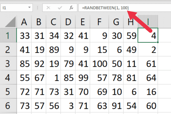
1. RANDBETWEEN Function
The RANDBETWEEN function is more flexible than RAND because you can specify the bottom and top numbers as something other than 0 and 1.
To generate data with numbers between 1 and 100, enter this formula into cell A1:

=RANDBETWEEN(1, 100)
Then, copy the cell to as many rows and columns as you want. It takes seconds to produce a grid of randomized numbers:
2. RANDARRAY Function
You may be thinking it would be nice to avoid the manual copy of the RANDBETWEEN function. To get super-advanced, you can use the new RANDARRAY function in the latest version of Microsoft Excel.
The syntax is:
RANDARRAY([rows], [columns], [min], [max], [whole number])
rows: number of rows
columns: number of columns
min: lowest number
max: highest number
whole number: defaults to TRUE, otherwise uses decimal numbers.
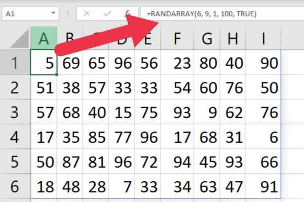
To generate random numbers between 1 and 100 across six rows and nine columns, use this formula:
=RANDARRAY(6, 9, 1, 100, TRUE)
Advanced Forecasting Formulas in Microsoft Excel
Excel’s forecasting functions are used for forecasting future values based on existing data trends. These functions help to identify patterns and project trends based on your data.
1. FORECAST.ETS Function
The older FORECAST function was replaced with a set of newer functions in Excel 2016.
You choose the function based on the specific forecasting model that you want. For example, the FORECAST.ETS function uses the Exponential Smoothing algorithm.
The syntax is:
FORECAST.ETS(target_date, values, timeline)
target_date: the date you want a calculated value for.
values: the historical data.
timeline: a range of dates
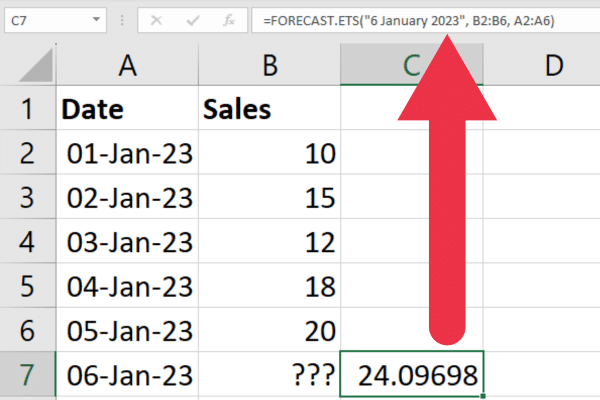
Suppose you have dates from the 1st to the 5th of January in column A and sales amounts in column B. This formula will predict the next sales amount:
=FORECAST.ETS(“6 January 2023”, B2:B6, A2:A6)
2. TREND Function
The TREND function projects a set of values based on the least squares method. It returns an array. The syntax is:
TREND(known_y, [known_x], [new_x], [const])
known_y: range of y values
known_x: range of x values
new_x: range of calculated values
Often, the known_y are the data points, while the known_x are the dates.
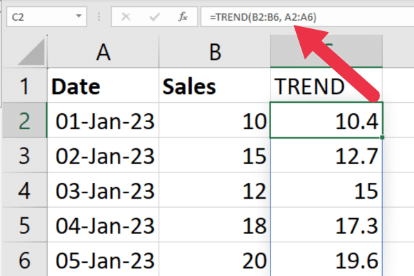
Using the same data as in the previous example, you can enter the below formula into cell C2. A set of values will be generated.
=TREND(B2:B6, A2:A6)
Advanced Statistical Formulas
The advanced statistical functions include calculating percentiles and quartiles. Some math functions are available for backward compatibility, but it’s recommended to use the most up-to-date versions.

1. PERCENTILE Function
This function calculates the percentage of data points that fall below a particular value. The syntax is:
PERCENTILE.INC(array, k)
array: the cell range
k: the percentile from 0 to 1
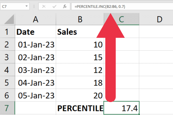
Suppose you want to calculate the 70th percentile of data in column B. Use this formula:
=PERCENTILE.INC(B2:B6, 0.7)
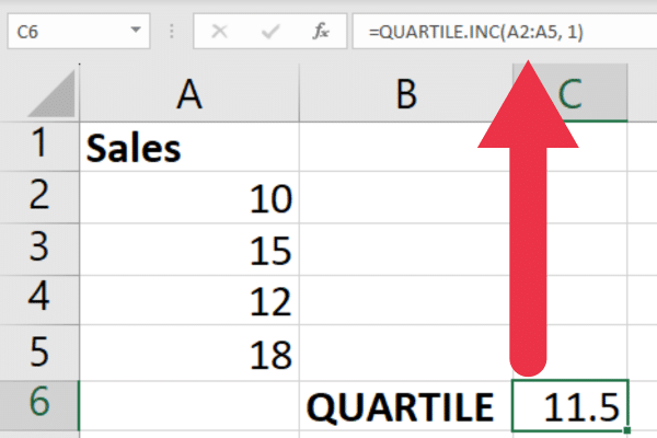
2. QUARTILE Function
This function is a variation of the percentile function but uses quarters to divide the data. This is the syntax:
QUARTILE.INC(array, quart)
array: the range of data
quart: 1 for the 25th percentile, 2 for the 50th, 3 for the 75th, and 4 for the maximum.
The formula below will calculate the first quartile of data in column A.
=QUARTILE.INC(A2:A5, 1)
Advanced Data Analysis And Manipulation Formulas
Several advanced functions let you switch the format of data, analyze frequency distributions, and extract data from pivot tables.
TRANSPOSE
FREQUENCY
GETPIVOTDATA
1. TRANSPOSE Function
Sometimes you want to move the data in your rows into columns and vice versa. You can do this manually or use the TRANSPOSE function instead.
Suppose you have the items “T-Shirt”, “Hoodie”, and “Jeans” in cells A2, A3, and A4. You want to make these into column headings. This function returns the values in a single row:
=TRANSPOSE(A2:A4)
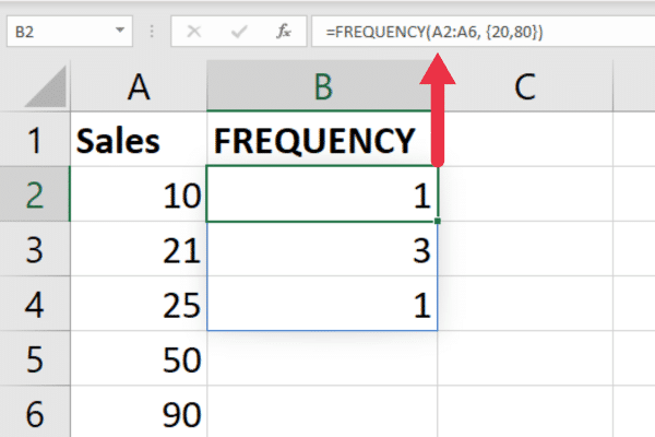
2. FREQUENCY Function
This function calculates the frequency distribution of values within a dataset. This is the syntax:
FREQUENCY(data_array, bins_array)
data_array: range of values.
bins_array: the intervals to use.
Suppose you have sales data in column B, and you want to analyze the frequency distribution of the values based on how many amounts are:
below 20.
from 20 to 80.
above 80.
That represents three bins and can be calculated with this formula:
=FREQUENCY(A2:A6, {20,80})
For more on frequency distributions in Excel, check out this video:
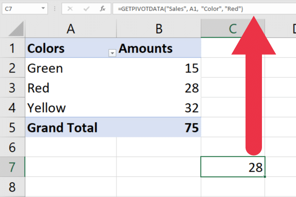
3. GETPIVOTDATA Function
This function lets you extract summarized information from pivot tables. This is the syntax:
GETPIVOTDATA(data_field, pivot_table, [field1, item1], [field2, item2], …)
data_field: the data field or value you want to retrieve from the pivot table.
pivot_table: a reference to the pivot table.
field1, item1, etc.: the field/item pairs to filter for.
Suppose you have a pivot table based on the color of items sold. To extract the sales for red items, use this formula:
=GETPIVOTDATA(“Sales”, A1, “Color”, “Red”)
Advanced Error Handling
Even the most basic Excel formulas can produce errors. Intermediate users should know how to use ISERROR to handle errors. Advanced users should also be familiar with the ERROR.TYPE function for error identification.
The ERROR.TYPE function helps identify the specific type of error within a cell or formula.
It returns a numeric value corresponding to different error types, such as #N/A, #VALUE!, #REF!, and more.
Suppose you have an error in cell A1 and you want to identify its error type. The following formula will return the number that corresponds to the specific error:
=ERROR.TYPE(A1)
You can combine this with multiple functions to respond differently depending on the type of error. These are the most common errors and their values:
#NULL! (no common cell found In a range)
#DIV/0! (division by zero or an empty cell)
#VALUE! (inappropriate data type or argument in a formula)
#REF! (a referenced cell has been deleted or there is a circular reference)
#NAME? (Excel doesn’t recognize the function or range)
#NUM! (invalid numeric value)
#N/A (value can’t be found)
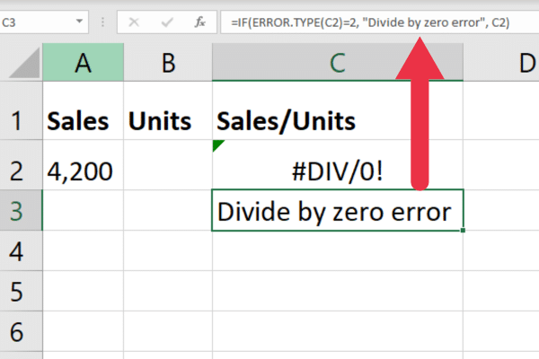
Suppose you want to handle three specific error types. Use this formula to display a specific error message based on the type:
=IF(ISERROR(C2), IF(ERROR.TYPE(C2)=2, “Divide by zero error”, IF(ERROR.TYPE(C2)=3, “Invalid value error”, IF(ERROR.TYPE(C2)=7, “Value not found error”, “Other error”))), C2)
Advanced Lookup Formulas
Our beginner and intermediate cheat sheets covered a selection of lookup functions. Here are some advanced options:
XLOOKUP
XMATCH
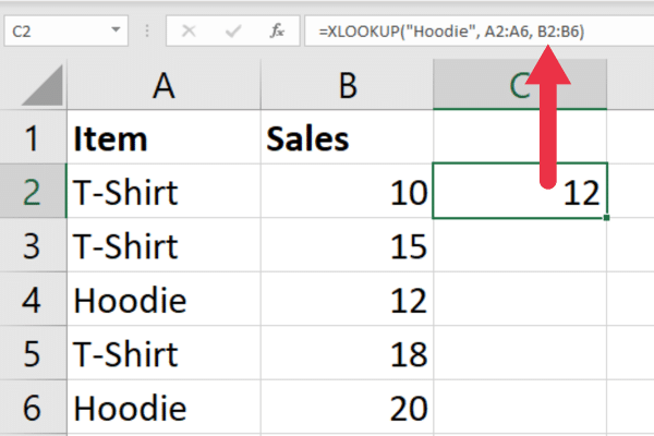
1. XLOOKUP Function
This lookup function allows you to search for a value in a range and return a corresponding value from another column or range.
It offers more versatility than simpler lookup functions like VLOOKUP. This is the syntax:
XLOOKUP(lookup_value, lookup_array, return_array, [match_mode], [search_mode], [if_not_found])
lookup_value: the value you want to search for.
lookup_array: the range for the lookup.
return_array: the range that will show the corresponding value.
match_mode: exact match (0), next smaller (1), next larger (-1), or wildcard match (2).
search_mode: -1 for top to bottom, 1 for bottom to top, or 2 for binary search.
if_not_found: sets the value to return if no match is found.
Suppose you want to search a range of data for the first occurrence of a clothes item and return the sales amounts. This formula will look for the text “Hoodie” and return the value in the adjacent cell if found:
=XLOOKUP(“Hoodie”, A2:A6, B2:B6)
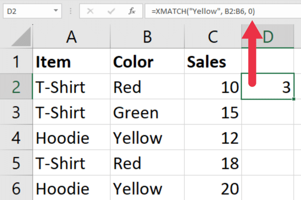
2. XMATCH Function
This function allows you to find the position of a specified value within a range or an array. This is the syntax:
XMATCH(lookup_value, lookup_array, [match_type], [search_mode])
lookup_value: the value you want to find.
lookup_array: The range you want to search.
match_type: exact match (0), next smallest (-1), next largest (1).
search_mode: binary search (1) or linear search (2).
Suppose you want to find the first occurrence of a yellow item in a range within column B. Use this formula:
=XMATCH(“Yellow”, B2:B6, 0)
Final Thoughts
This cheat sheet has covered a wide range of functions, from statistical analysis, lookup formulas, data manipulation techniques, and error handling strategies.
The provided examples and explanations help demystify these advanced formulas, making them accessible even to those with limited experience.
As you start to incorporate them into your Excel tasks, you are on your way to increasing your Excel skills to an advanced level.
But remember, this cheat sheet is just the tip of the iceberg. The really amazing stuff happens when you get creative, mix and match these formulas, and tailor them to solve your unique challenges. Excel is like a canvas, and these formulas are your palette — so go ahead, paint your masterpiece!


