
In Excel, the “does not equal” symbol is called a logical operator. This powerful tool allows you to quickly and efficiently compare values within your spreadsheet and make decisions based on their differences.
By understanding how to utilize the “does not equal” symbol, you can enhance your Excel skills and create more advanced formulas.
The “does not equal” symbol in Excel is denoted by the pair of angled brackets pointing away from each other, like this: “<>”. When Excel encounters this sign in your formulas, it will assess whether the two statements on each side of the symbol are equal. If they are not equal, Excel will return TRUE; otherwise, it will return FALSE.


Learning how to effectively use the “<>” symbol in Excel can be a valuable addition to your spreadsheet skills.
Moreover, Familiarizing yourself with this operator and other logical functions will help you create more sophisticated formulas that can handle complex data analysis tasks with ease.
So, let’s dive in and discover the magic of the “does not equal” sign to take your Excel game to the next level!
Understanding the Not Equal Symbol
The Not Equal to operator in Excel is a comparison operator that plays a crucial role in making logical comparisons between values, such as numbers, text, or dates. Represented by the symbols <>, this sign helps you verify if two values are distinct.
If the compared values aren’t equal, the result is TRUE.
Otherwise, it returns FALSE.
In Windows and Microsoft Word, there are several shortcuts for you to enter? Such as using a character map etc.
But, while there’s no dedicated keyboard shortcut for this specific symbol in Excel, it’s relatively straightforward to enter this symbol.

Use the Not Equal Sign with Different Data Types
When working with Excel, the Not Equal sign is a powerful tool for comparing values, strings, or characters.
Here’s how you can use the Not Equal sign with different types of data:
Numbers:
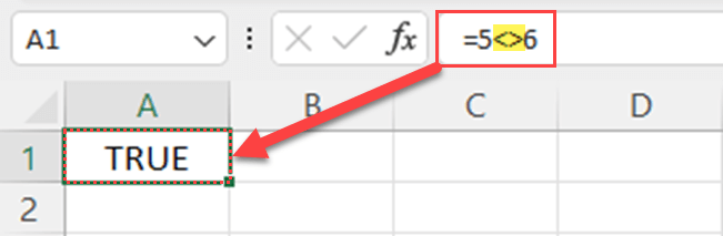
When comparing numeric values, simply insert the operator between the two numbers. For instance, the formula =5<>6 will return TRUE, indicating that the two numbers are not equal.
Text:
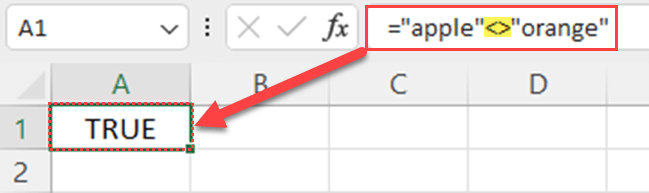
To compare textual values, use the Not Equal sign. For example, the formula =”apple”<>”orange” will return TRUE because the two texts are distinct.
Dates:
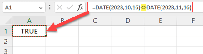
Similar to numbers and text, use the Not Equal symbol within two dates to determine if they are different. For example, =DATE(2023,10,16)<>DATE(2023,11,16) will result in TRUE, signifying that the two dates are not equal.
Using Not Equal Symbol in a Basic Formula
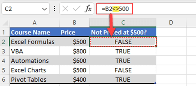
Compare a particular cell value
Imagine you have a list of course prices, and you want to find the courses that don’t cost $500. To do this using the Not Equal symbol, enter this formula into a blank cell:
=B2<>500
When you press Enter, the formula will give you either a TRUE or FALSE answer, depending on whether the course price is not $500. Just copy this formula down the column to compare prices for each course.
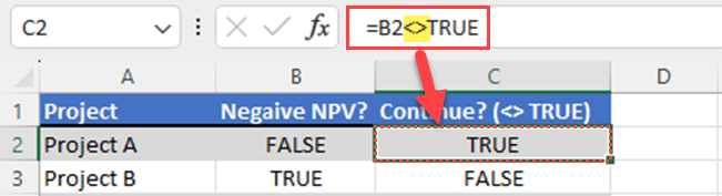
Compare Logical Values (Boolean Values)
If you need to check if a cell’s value is not equal to a TRUE or FALSE statement, you can use the following formula format:
=B2<>TRUE
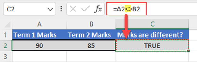
Compare Selected Cells
Another common usage of the Not Equal to operator is to compare values across cell references or a cell range. If you want to compare two different cells, say A2 and B2, the formula would be:

=A2<>B2
This formula will return a TRUE result if the values are not the same and a FALSE result if they are equal. Please refer to the below screenshot.
It is important to note that when comparing text, the Not Equal sign is case-insensitive, meaning “ORANGES” and “oranges” are treated as equal.
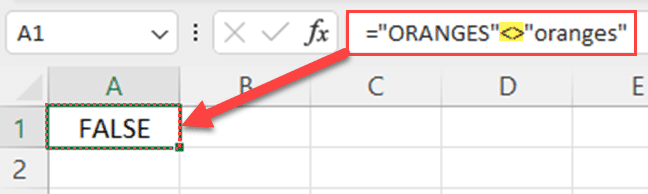
In the above formula, Excel considers the two values to be identical, even though one of them has letters in uppercase.
In conclusion, with a confident and knowledgeable approach, you can apply the Not Equal to Operator (<>) in Excel formulas.
Practical Examples and Results
In this section, you’ll learn practical examples of using the “does not equal” (<> or ?) symbol in Excel functions.
These examples will provide you with a clear understanding of how this powerful operator can be used effectively in your spreadsheets.
Example 1: Grading Students
Suppose you have a list of students and their grades. You want to analyze students who did not receive a specific grade, say “E”.
To do this, you can use the IF function combined with the “does not equal” symbol:
=IF(B2<>"E", "Passed", "Failed")
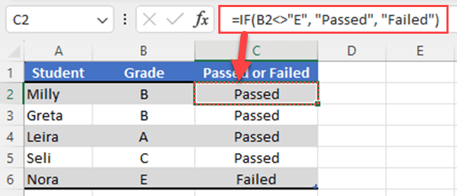
Here, B2 contains the grade, and if the grade isn’t equal to “E”, the formula returns “Passed”, otherwise, it returns “Failed”.
Example 2: Summing Values Based on a Condition
You may encounter situations where you need to sum cells that do not meet specific criteria. The SUMIF function can be used in conjunction with the “does not equal” symbol.
Let’s say you have a dataset of sales and you want to calculate the total sales that are not from a particular region, like “East”.
=SUMIF(B2:B6, "<>East", C2:C6)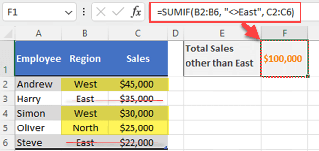
In this example, the formula calculates the sum of values in the sales column (Column C) where the corresponding region in column A does not equal “East”.
Example 3: Filtering Data Based on Criteria
The “does not equal” symbol can be especially useful when filtering data in a spreadsheet.
If you have a sales dataset and you want to extract the rows that don’t belong to the East region, you can apply the FILTER function to test and filter data.
=FILTER(A3:C7,B3:B7<>"East")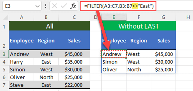
These examples demonstrate how the comparison operators such as the “does not equal” symbol can be a versatile tool in Excel, helping you achieve various goals in your data analysis and management tasks.
Conditional Formatting with Not Equal Sign
Conditional formatting allows you to automatically apply different formats to cells based on their content.
In Excel and other spreadsheet software like Google Sheets, you can use the not equal sign (<>) for conditional formatting rules.

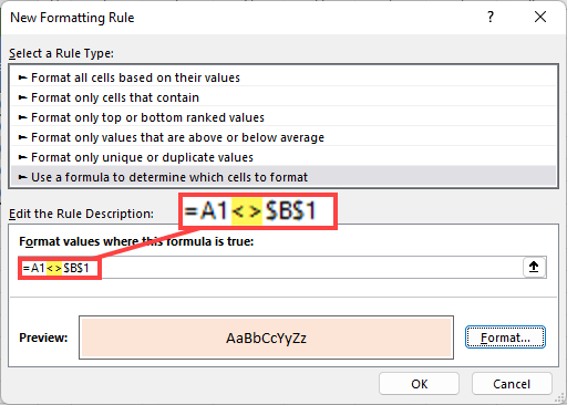
To apply conditional formatting using the not equal sign, follow these steps:
Select the cells you want to apply the conditional formatting.
Navigate to the Home tab, click on Conditional Formatting, and then choose New Rule.
In the New Formatting Rule window, select “Use a formula to determine which cells to format”.
In the Formula field, enter the comparison formula using the not equal sign (<>). For example, if you want to highlight cells in column A that are not equal to the value in B1, enter =A1<>$B$1.
Click on Format and choose the desired format (e.g., background color, font style, etc.).
Click OK to apply the conditional formatting rule.
In case you’re using Microsoft Excel on a Mac, the process is almost identical, as the Home tab, Conditional Formatting, and New Rule options are all present in the Mac Excel interface.
Make sure to use the dollar sign ($) for absolute references in your formulas when necessary. This ensures that the formatting rule doesn’t change when applied to other cells in the range.
By using the not equal sign within your conditional formatting rules, you can easily highlight discrepancies in your data. This can aid in quickly identifying potential issues and making your data more comprehensible.
Final Thoughts
Now that you’ve got the hang of typing “not equal” in Microsoft Excel, you can use it with different types of information. You can also use does not equal symbol and other logical operators in simple math formulas and more complex things like IF, SUMIF, and FILTER.
And don’t forget, it can also help you make your data stand out with special formatting rules. You’re all set to excel in Excel!
Are you interested in diving into the world of analytics tools?
See how traditional platforms like Power BI and Excel stack up against the advanced AI features of Code Interpreter in the video below.
Frequently Asked Questions
How to apply not equal to in Excel formulas?
To apply the “Not Equal to” operator in Excel formulas, use the symbol “<>”. Simply type an equals sign “=” in the cell, you want to return the result, select the cell you want to compare, and then type the “Not Equal to” operator followed by the value or cell you want to compare it with. For example: =A1<>B1
How to use the COUNTIF function with not equal criteria?
You can use the COUNTIF function with a “Not Equal to” operator to count the number of occurrences that a condition that is not met in a range. Syntax: =COUNTIF(range,”<>criteria”). For example: =COUNTIF(A1:A10, “<>Apple”) would count cells in the range A1 where the value does not equal “Apple.”
How to implement SUMIF with a does not equal condition?
The SUMIF function can be used with a “Not Equal to” operator to sum cells that do not meet the specified criteria. Syntax: =SUMIF(range, “<>criteria”, [sum_range]). For example: =SUMIF(A1:A10, “<>10”, B1:B10) would sum the cells in range B1 where the corresponding cell in range A1 does not equal 10.
How to filter cells that are not blank in Excel?
To filter cells that are not blank in Excel, use the “Not Equal to” operator with an empty string “”. In the filter dropdown, select “Custom Filter” and choose “Does not equal” as the condition, then enter “” in the criteria box. This will filter all the cells containing values and exclude the blank ones.
How to use NOT function with OR in Excel?
The NOT can be used with the OR function to check whether one or more conditions are not met. Syntax: =NOT(OR(condition1,condition2,…)). For example: =NOT(OR(A1=”Red”, B1<5)) would return TRUE if neither A1 is “Red” nor B1 is less than 5.
How to write a conditional statement for not equal to zero?
To write a conditional statement for a value in a cell not equal to zero, use the “Not Equal to” operator with an IF function. Syntax: =IF(cell<>”0″,value_if_true, value_if_false). For example: =IF(A1<>0, “Non-zero”, “Zero”) would output “Non-zero” if A1 is not 0, and “Zero” if A1 is 0.


