
Want to create Pivot Tables using data from all over the place without cramming it into one Excel file? Well, you’re in luck with Excel’s superhero sidekick, Power Pivot!
Power Pivot helps you work with big loads of data from different places, making it easy to understand and find insights. You can create data models, make connections, and perform powerful data analysis, all in the regular Excel you’re used to. Just turn it on through Excel’s options, and you’re good to go.
Excel Power Pivot is like your secret weapon for handling big data. It’s a game-changer for businesses, helping you dig deep into data and make smart decisions.

So, are you ready to take your data skills to the next level?
Let’s dive in!

How to Activate Excel Power Pivot Tab
To enable Power Pivot in Microsoft Excel, follow these simple steps:
Step 1
Click File > Options > Add-Ins.
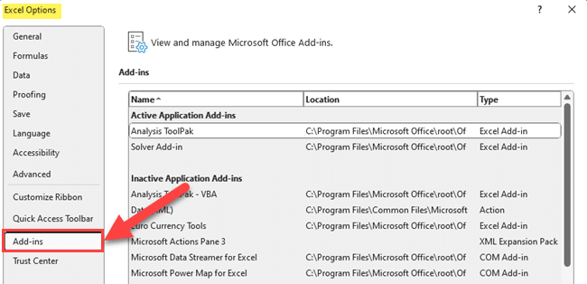
Step 2

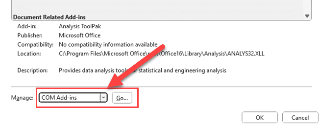
Select COM Add-Ins from the Manage list, and click Go.
Step 3
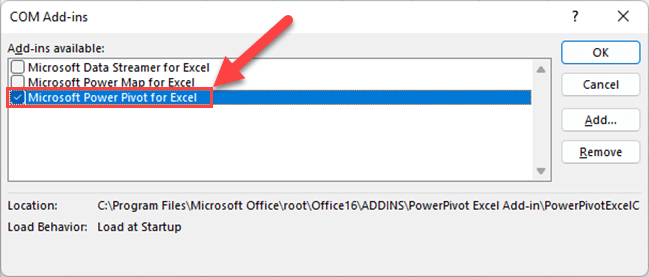
Check the box for Microsoft Power Pivot for Excel and click OK.
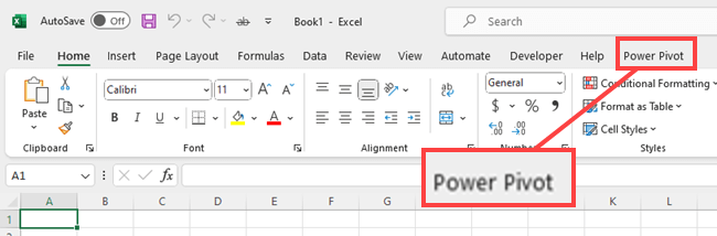
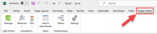
The Power Pivot tab will then be visible on the Ribbon.
Once you’ve activated Excel Power Pivot, you can get data from different sources, transform raw data into meaningful information, and build interactive and visually appealing dashboards. T
Basics of Power Pivot
Power Pivot is an Excel add-in that helps you analyze big data easily. You can create sophisticated data models by bringing in data from different places and linking it together. It works in Excel versions from 2010 and later, including Excel for Microsoft 365.
As you begin using Power Pivot, you’ll first import data into tables. These tables can be connected by defining relationships that link related columns. This interconnected set of tables forms a data model, providing you with a comprehensive view of your information.
How to Import Data to the Power Pivot Model
To import data into your Power Pivot workbook, follow these simple steps:
Step 1
Go to the Power Pivot tab.
Step 2
Click Manage.
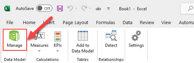
Now Excel will open the Power Pivot window.

Step 3
Go to the Get External Data section and select your data sources.

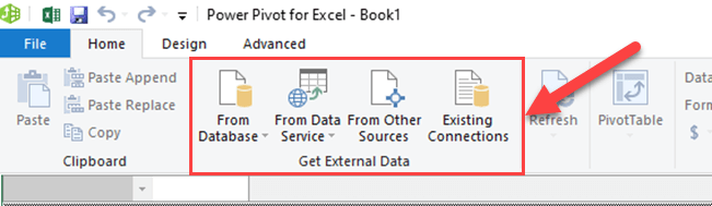
This allows you to connect to various sources such as SQL Server relational databases, Microsoft Access databases, ATOM data feeds etc. When importing data, you have the option to filter out any unnecessary information, rename tables and columns, and import relationships between tables.
You can also take advantage of Power Query, an integrated feature within Excel that complements Power Pivot.
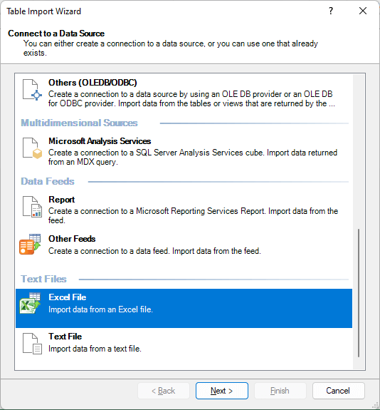
If you want to import Excel Tables, click “From Other Sources” and select “Excel File” under the “Text Files” of the Table Import Wizard.
How to Build Relationships Between Tables?
Once your data is imported, you can create relationships between tables to establish a useful data model. You do this by:
Step 1
Go to the Diagram View in the Home tab of the new window.
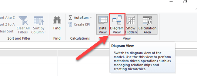
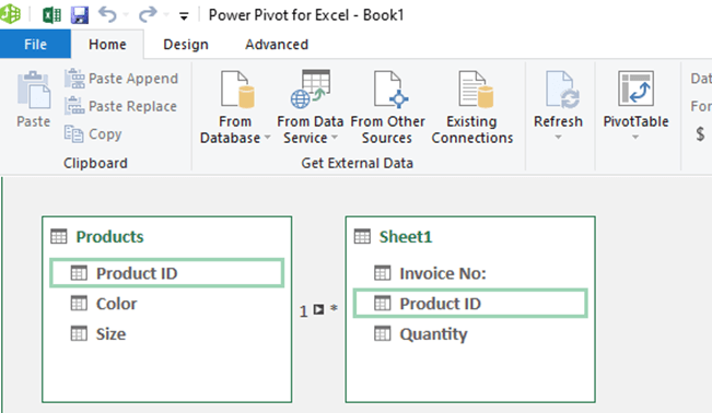
Step 2
Dragging a field from one table onto its related field in another table. A line will appear to visualize the relationship.
With your data model in place, you can leverage Power Pivot’s powerful capabilities, such as Data Analysis Expressions (DAX) formulas, to create custom calculations and measures.
By combining large volumes of data from multiple sources and applying advanced calculations, you can gain valuable insights into your data and make more informed decisions.
Now that you’re familiar with the basics of Power Pivot, explore its features and benefits to unleash the full potential of data analysis in Excel.
The Interface and Tools
Working with Excel Power Pivot is a seamless experience, as its interface is integrated into the Excel environment. You can access Power Pivot through the Ribbon.
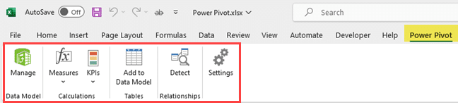
Power Pivot introduces a set of new tools that can greatly enhance your data analysis capabilities. Some key features you will find within the Power Pivot ribbon include:
Manage: Opens the Power Pivot window where you can modify the Data Model, create relationships, and work on calculations.
Add to Data Model: Allows you to add new tables to your Data Model from a variety of data sources.
Measures: Provides tools for creating and managing custom calculations or measures using the DAX language.
KPIs: Enables you to create Key Performance Indicators based on your data to track performance and goals.
Relationships: Allows you to define the relationships between tables in your Data Model, making it easier to work with related data.
By understanding and utilizing the interface and tools provided by Power Pivot, you can enhance your data analysis capabilities and unlock the full potential of your data.
How to Create Calculations in Power Pivot
In Excel Power Pivot, you can make your data work better by doing math on it. You can do this in a few ways:
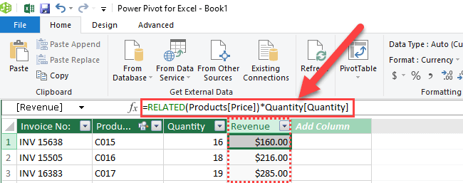
1.) Calculated Columns: You can add new columns to your data by writing down special math formulas. Each row in your data will get a new value based on these formulas. It’s like creating new columns of information from the existing ones.
2.) Calculated Fields (Measures): These are like super math calculations used in tables. They are used for complex things like finding the total or average of your data. You write down special formulas to do these calculations.
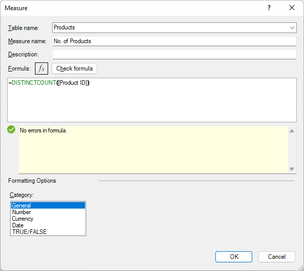
In Power Pivot, we use a special math language called DAX. It’s similar to regular Excel formulas, but it’s more powerful and can handle complex data relationships.
Remember, to do this, you need to understand your data, how it’s connected, and how to write these special math formulas. Once you get the hang of it, you can use Power Pivot to make your data tell you important things about your business
How to Create KPIs in Power Pivot
In a Power Pivot data model, you can make Key Performance Indicators (KPIs) to measure how well a business metric is doing. To create KPIs, you pick a starting value, set a goal, and choose a symbol to show progress.

Here’s how to make KPIs in Power Pivot:
Select a Measure: Pick a calculated measure you want to use as the starting point for your KPI. This measure helps you evaluate your performance.
Create a New KPI: Go to the Power Pivot tab and click on ‘KPIs,’ then ‘New KPI.’ A box will pop up.
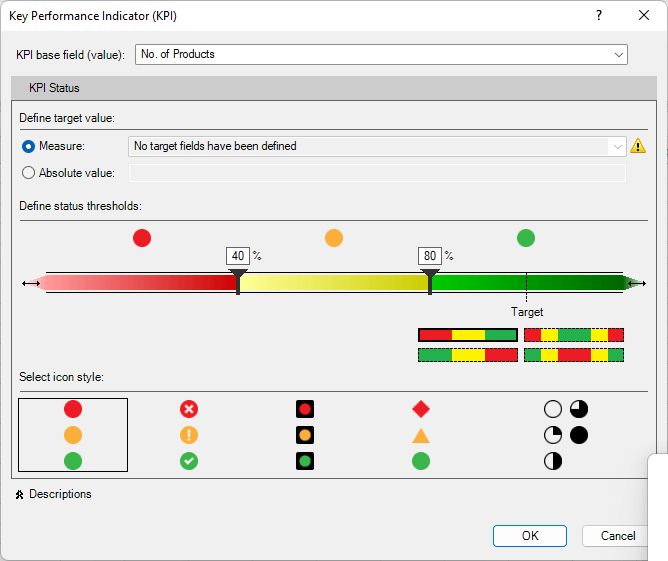
Define the KPI Base Field: Choose the measure you picked earlier as your KPI’s starting point. This is the value that the KPI will use to see how well you’re doing compared to your goal.
Set the Goal: You can type in a specific number as your goal or use another measure as your goal. The KPI will compare your progress against this goal.
Choose a Symbol: You can pick a symbol to show whether you’re meeting the goal, falling short, or exceeding it.
Save the KPI: After you’ve set everything up, click ‘OK’ to save your KPI.
Once your KPI is ready, you can use it in your data analysis, PivotTables, and Power View reports. KPIs help you quickly see where your performance is strong or needs improvement, so you can make smart decisions for your business.
How to Create PivotTables and PivotCharts
When working with Excel, you might encounter large data sets that require analysis and visualization. Two powerful tools that can help you with this task are PivotTables and PivotCharts. PivotTables allow you to summarize and analyze your data, while PivotCharts provide a visual representation of that data, making it easier to spot trends and patterns.
To create a PivotTable using the Data Model, follow these steps:
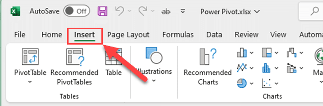
Step 1
Go to the Insert tab in the Excel Ribbon.
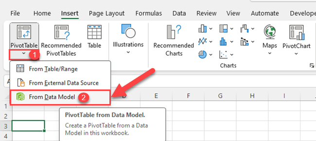
Step 2
Expand PivotTable options and select “From Data Model”.
Step 3
Choose where you’d like the PivotTable to be placed, either a new or existing worksheet.
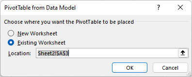
Step 4
Click OK to create the PivotTable.
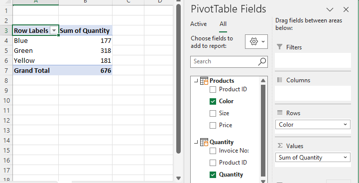
Once you’ve created a PivotTable, you can adjust its layout, add filters to better understand your data, and explore different summaries and calculations.
Similarly, to create a PivotChart, follow these simple steps:
Step 1
Click on any cell within the created PivotTable.
Step 2
Go to the Insert tab in the Excel toolbar.
Step 3
Click the PivotChart icon.
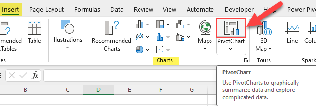
As you do this, the Create PivotChart dialog box appears.
Step 4
Choose the chart type you prefer for your data representation.
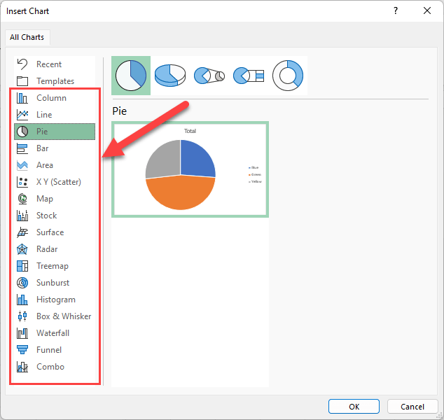
Step 5
Click OK to create the PivotChart.
Now you have a visual representation of your PivotTable data. PivotCharts makes it easy to share and understand the insights you’ve gathered from your analysis.
With PivotTables and PivotCharts at your disposal, you have the tools necessary to make informed decisions based on your data.
Next up, let’s tackle this commonly asked question.
Are Power Pivot and Power BI the Same Thing?
Power Pivot in Excel:
Great for handling large datasets.
Allows you to create data relationships.
Performs complex calculations.
All within the familiar Excel environment.
Power BI:
A comprehensive tool for data visualization and reporting.
Combines Power Pivot and Power Query for enhanced data management.
Ideal for creating visual reports and dashboards.
Facilitates easy sharing of insights.
Combining Both Tools:
Use Power Pivot in Excel for data modeling and heavy lifting with data.
Use Power BI for advanced data visualization, making data more appealing and shareable.
The combination streamlines data analysis and helps derive valuable insights.
In summary, Excel Power Pivot specializes in data modeling and calculations, while Power BI focuses on data visualization and reporting.
By leveraging the strengths of both tools, you can efficiently manage, analyze, and visualize your datasets to make informed decisions for your organization.
What is Time Intelligence in Power Pivot?

Time Intelligence in Power Pivot is a potent tool for analyzing data over time, great for tasks like forecasting and tracking cumulative sales.
To use it effectively, you’ll need a date table with a well-organized sequence of dates, ensuring comprehensive data analysis. Functions like TOTALYTD, DATESYTD, and others help you analyze data across various time periods.
To make the most of these tools, you should get familiar with Data Analysis Expressions (DAX) and explore different time intelligence functions. This knowledge enables you to create informative reports that offer insights into your business’s performance over time.
Final Thoughts
Great! You’ve learned how to bring the Power Pivot tab into Excel, and that’s like unlocking a unique tool. It lets you connect lots of different data sources, which is like gathering information from other places.
With this fantastic tool, you can do thorough data analysis using Pivot tables and Pivot charts, which are innovative ways to organize and show your data. It’s kind of like having a superpower for handling data in Excel!
If you’re interested in understanding how to utilize variables in your DAX formula with Power BI, be sure to check out the video below!
Frequently Asked Questions
How to enable Power Pivot in Excel?
To enable Power Pivot in Excel, follow these steps:
Open Excel and click on ‘File.
Select ‘Options’ from the drop-down menu.
Navigate to the ‘Add-Ins’ tab.
Locate ‘COM Add-ins’ in the ‘Manage’ drop-down menu and click ‘Go’.
Check the box next to ‘Microsoft Power Pivot for Excel’ and click ‘OK’. Power Pivot is now enabled, and you will see a new tab in your Excel toolbar.
What are some Power Pivot examples?
Power Pivot provides powerful data modeling and analysis in Excel. Some examples include:
Combining multiple data sources into a single report or analysis.
Creating complex calculations, such as time-based comparisons or moving averages.
Analyzing large volumes of data rapidly and efficiently.
How to add a Power Pivot Data Model in Excel?
Once you have enabled Power Pivot, follow these steps:
Click on the ‘Power Pivot’ tab in your Excel toolbar.
Select ‘Manage Data Model’ to open Power Pivot.
In the Power Pivot window, click on ‘Home’ followed by ‘Get External Data’.
Choose your data source and import the data into Power Pivot.
Create relationships, calculations, and pivot tables based on the imported data.
What is the difference between a Power Pivot and a normal pivot?
The main difference between Power Pivot and normal pivot tables is that Power Pivot offers advanced data modeling capabilities and allows for the integration of multiple data sources. Power Pivot also enables users to perform complex calculations and perform faster data analysis on large volumes of data. In contrast, normal pivot tables typically operate with a single data source and provide more basic data analysis.
Is Power Pivot worth learning?
Yes, learning Power Pivot can be extremely beneficial if you work with large volumes of data from various sources and need to perform complex calculations or analysis. Gaining a solid understanding of Power Pivot will allow you to create sophisticated data models, improve your analysis capabilities, and ultimately, enhance your overall efficiency in Excel.
Is Power Pivot free for Excel?
Power Pivot is included as a free, built-in feature in certain versions of Excel, such as Excel 2013, 2016, 2019, and Microsoft 365. It is not available in Excel 2010 by default but can be installed as an add-in. If you have one of the mentioned Excel versions, you can enable Power Pivot without any additional cost.


