
When working with large sets of data in Microsoft Excel, it can be challenging to find multiple values that match several conditions. Some built-in functions, e.g. VLOOKUP, were originally designed to work with single values.
Several Excel functions can be combined to lookup multiple values. They include VLOOKUP, INDEX, MATCH, and IF functions. Current versions of Excel can use dynamic arrays while older versions use array formulas.
This article will show you exactly how to use these functions in formulas that find multiple values in your data.

Let’s go!
How to Use VLOOKUP with Multiple Values
The VLOOKUP function is often used to find single values in a range of data. However, you can also look up multiple matches in Excel with this lookup formula.
By default, it will only return the first matching value it finds. However, you can modify the function to return multiple values by using an array formula.
What are Array Formulas?
An array formula is a formula that can perform calculations on arrays of data. It’s called an array formula because it can return an array of results, rather than a single value.
There are several easy steps when creating an array formula:
Select a range of cells to search.
Enter the formula in the formula bar.
Press Ctrl + Shift + Enter to complete it.
The syntax of an array formula is similar to that of a regular formula, but it includes curly braces {} around the formula. The curly braces indicate that the formula is an array formula and that it will return an array of values.

The examples in this article will show you how to use array formulas correctly.
VLOOKUP Example
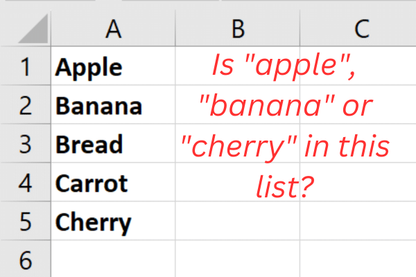
Our example has five items in column A of a worksheet:
Apple
Banana
Bread
Carrot
Cherry
The task is to check if three specific fruits are in this list: apple, banana, and cherry.
Latest Versions of Excel
The VLOOKUP syntax depends on which version of Excel you are using.
The most recent versions (Excel 365 or Excel 2021) support dynamic arrays. This feature allows formulas to return multiple results that “spill” into adjacent cells.
This is the syntax (the equal sign starts the formula):
=VLOOKUP(lookup_value, table_array, col_index_num, [range_lookup])
lookup_value: The value that you want to look up.
table_array: The entire data table that you want to search.
col_index_num: The table column number in the table_array that contains the data you want to return.
range_lookup: Optional. Specifies whether you want an exact match or an approximate match.
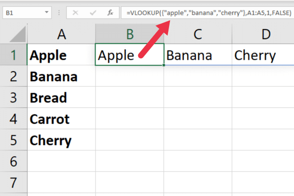
Our specific example uses this formula:
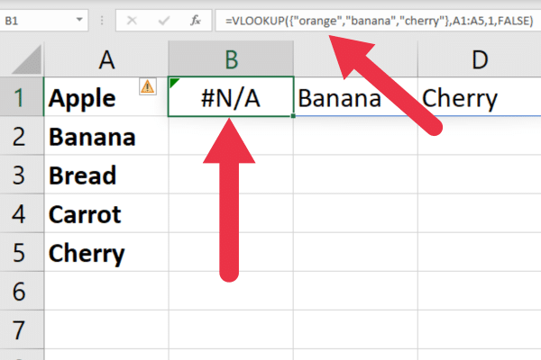
=VLOOKUP({“apple”,”banana”,”cherry”},A1:A5,1,FALSE)
When the formula is entered in cell B1, the results spill into cells C1 and D1. This picture shows the example in action:
Older Versions
If you’re using an older version of Excel that doesn’t support dynamic arrays (e.g., Excel 2019 or earlier), you’ll need to use a slightly different approach with an array formula.
Follow these steps:
Click on the cell where you want to display the results for the first item (e.g., column B).
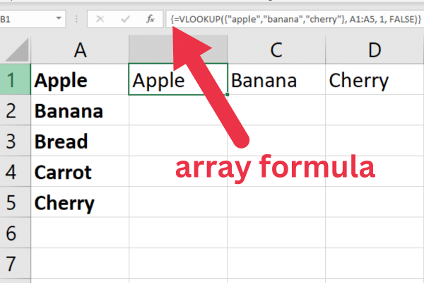
Type the following formula without pressing Enter yet: =VLOOKUP({“apple”,”banana”,”cherry”}, A1:A5, 1, FALSE)
Press Ctrl + Shift + Enter to turn this into an array formula.
Copy cell B1 and paste it into the cell below (or use the fill handles).
When you use Ctrl + Shift + Enter, Excel adds curly braces around the formula. This indicates that it is an array formula.
Exact Match vs. Approximate Match
By default, the VLOOKUP function uses an approximate match. This means that it will return the closest match it can find, even if the cell values are not an exact match.
If you want to perform an exact match, you can set the range_lookup argument to FALSE.

Bear in mind that approximate matches work best with ordered numerical values. It is usually not appropriate when the cell value is text.
More About VLOOKUP
If you want to learn more about this versatile function, check out these articles:
Now that you’re set with the VLOOKUP function, let’s take a look at two other functions that can do what it does in a different way: INDEX and MATCH.
How to Use INDEX And MATCH to Lookup Multiple Values
You can combine the INDEX and MATCH functions together to find multiple values in multiple rows.
The INDEX function in Excel returns a value or reference to a cell within a specified range.
=INDEX(array, row_num, [column_num])
array: The range of cells to be searched for the value.
row_num: The row number within the array from which to return a value.
column_num: (Optional) The column number within the array from which to return a value. If omitted, the function returns the entire row.
The MATCH function in Excel returns the position of a value within a specified range.
=MATCH(lookup_value, lookup_array, [match_type])
lookup_value: The value to be searched for within the lookup_array.
lookup_array: The range of cells to be searched for the lookup_value.
match_type: (Optional) The type of match to be performed. If omitted, the function performs an exact match.
How to Use INDEX and MATCH Together in Excel 365
To use INDEX and MATCH together to look up multiple values in Excel, you need to use an array formula.
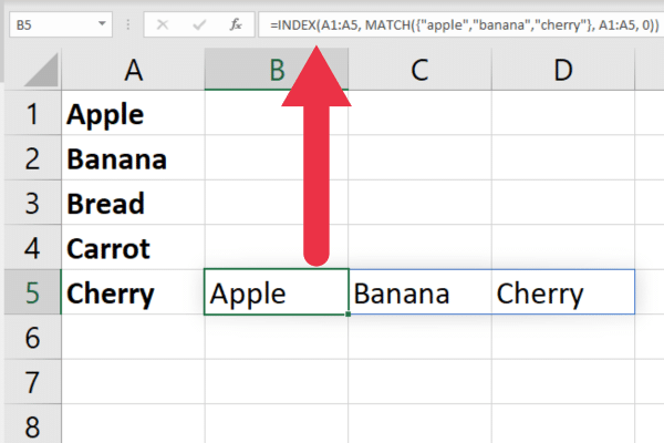
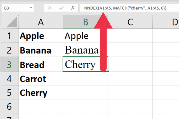
Working with the earlier sample data, this is the formula in Excel 365:
=INDEX(A1:A5, MATCH({“apple”,”banana”,”cherry”}, A1:A5, 0))
The above example breaks down as this:
INDEX: this returns the value of a cell in a specified range based on a given row and column number. In this case, it will return the value from the range A1:A5.
A1:A5: This is the defined table range where you’re searching for the value and from which the result will be returned.
MATCH: this searches for a specified item in a range of cells and returns the relative position of that item in the range.
{“apple”,”banana”,”cherry”}: this is the array constant containing the values you want to look up.
A1:A5: this is the range where MATCH will search for the values from the array constant.
0: this is the match type for MATCH function. In this case, it’s 0, which means you’re looking for an exact match instead of a close match.
This picture shows the formula in action:
Working with Older Versions of Excel
If you’re using an older Excel file that doesn’t support dynamic arrays (e.g., Excel 2019 or earlier), you’ll need to use a different approach.
Because older versions don’t support the formulas “spilling” into adjacent cells, you will need to break out the usage into three separate formulas.
Follow these steps:
Click on the cell where you want the result for the first item (e.g., cell B1)
Type the below formula:
=INDEX(A1:A5, MATCH(“apple”, A1:A5, 0))
Press Enter to execute the formula.
Type this formula in cell B2: =INDEX(A1:A5, MATCH(“banana”, A1:A5, 0))
Type this formula in cell B3: =INDEX(A1:A5, MATCH(“cherry”, A1:A5, 0))
This picture shows cell reference B3:
INDEX and MATCH functions aren’t the only ones that can enable you to find multiple values. In the next section, we look at how you can use the IF function as an alternative.
How to Use the IF Function to Find Multiple Values
Another way to lookup multiple cell values based on certain criteria is to use the IF function with other functions.
The IF function allows you to test multiple conditions and return different results depending on the outcome of those tests.

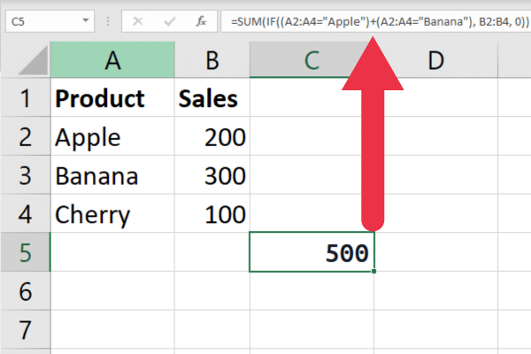
For example, let’s say you have a table of sales data with columns for Product and Sales. You want to lookup and total the sales amount for two of the three products.
Current Versions of Excel
To find the sum of the Sales column where the product is either “Apple” or “Banana” using the IF function, you can use an array formula with IF, SUM, and OR functions.
Assuming your data starts in cell A1, use the following formula:
=SUM(IF((A2:A4=”Apple”)+(A2:A4=”Banana”), B2:B4, 0))
The section (A2:A4=”Apple”)+(A2:A4=”Banana”) creates an array that has a value of 1 if the cell in range A2:A4 contains “Apple” or “Banana”, and 0 otherwise.
The IF statement checks each element of the array argument. If the value is 1 (i.e., the product is either “Apple” or “Banana”), it takes the corresponding value in the Sales column (range B2:B4); otherwise, it takes 0.
The SUM function adds up the values from the IF function, effectively summing the sales values for both “Apple” and “Banana”.
This picture shows the formula in action on the search range:
Older Versions of Excel
In Excel 2019 or earlier, you need to use an array formula. Follow these steps:
Type the formula but do not hit Enter.
Press Ctrl + Shift + Enter to make it an array formula.
Excel will add curly brackets {} around the formula, indicating it’s an array formula.
Next, we look at how you could use SUMPRODUCT to lookup several values based on your criteria. Let’s go!
How to Use SUMPRODUCT for Multiple Criteria
The SUMPRODUCT function also allows you to lookup multiple values based on multiple criteria.
Because it does not require the use of an array formula, the syntax is the same regardless of the version of Excel.
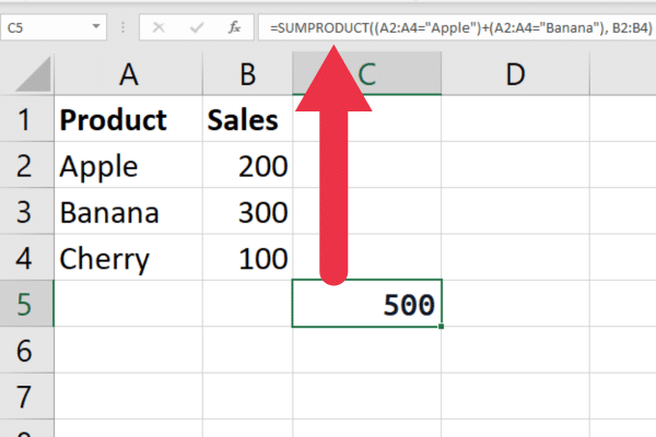
Using the same data as in the previous example, the formula looks like this:
=SUMPRODUCT((A2:A4=”Apple”)+(A2:A4=”Banana”), B2:B4)
The section (A2:A4=”Apple”)+(A2:A4=”Banana”) creates an array that has a value of 1 if the cell in range A2:A4 contains “Apple” or “Banana”, and 0 otherwise.
The SUMPRODUCT function multiplies the elements of the array with the corresponding elements in the Sales column (range B2:B4). It then adds up the resulting values, effectively summing the sales values for both “Apple” and “Banana”.
The below formula shows it in action:
Excel functions are amazing when they work as expected, but sometimes you may run into errors. In the next section, we cover some of the common errors and how you can deal with them.
3 Common Errors with Lookup Functions
Lookup functions can sometimes return errors that can be frustrating and time-consuming to troubleshoot. The three most common errors you will encounter are:
#N/A Errors
#REF! Errors
Circular Errors
1. #N/A Errors
The #N/A error occurs when the lookup value cannot be found in the lookup array.
There are several reasons why this error may occur, including:
the lookup value is misspelled or incorrect.
the lookup array is not sorted in ascending order.
the lookup value is not in the data set.
When the lookup value is not in the data set, this is useful information. However, inexperienced Excel users may think that #N/A means something has gone wrong with the formula. The next section shows how to make this more user-friendly.
2. #REF! Errors
The #REF! error occurs when the lookup array or return array is deleted or moved.
This error can be fixed by updating the cell references in the lookup function.
3. Circular Errors
As you combine functions in complex formulas, Excel may tell you that you have a circular reference.
You’ll find these easier to investigate by using our guide to finding circular references in Excel.

How to Use IFERROR with Lookup Functions
The IFERROR function is a useful tool for handling errors in lookup functions. It allows you to specify a value or formula to return if the lookup function returns an error.
The syntax for the IFERROR function is as follows:
=IFERROR(value, value_if_error)
· value: value or formula you want to evaluate.
· Value_if_error: the value or formula to return if the first argument returns an error.
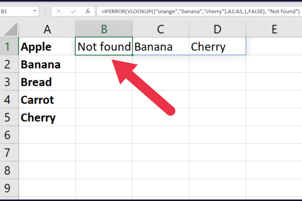
For example, let’s say you have a VLOOKUP function that is looking up multiple values in a table. In the picture below, one of the values does not exist in the searched data range.
As you can see, the #N/A error is displayed, which can be confusing to inexperienced Excel users.
Instead, you can use IFERROR to display a blank cell or a message that says “Not found” with this syntax:
=IFERROR(VLOOKUP(lookup_value, table_array, column_index, FALSE), “Not found”)
In this example, if the VLOOKUP function returns an error, the IFERROR function will return the message “Not found” instead.
This picture shows the formula in action. Column B has the missing value, while column C and column D have found matches.
We’ve covered a lot of ground so far, and you’re finally ready to learn more advanced techniques for lookups, which is the topic of the next section.
7 Advanced Lookup Techniques
Looking up multiple values in Excel can be a challenging task, especially when dealing with large datasets. You may encounter performance issues with slow processing.
There are seven advanced lookup techniques you can use to make the process easier and more efficient.
Relative position lookup
SMALL function
ROW function
FILTER Function
Helper columns
Dynamic Arrays
Power Query
1. Relative Position Lookup
One of the simplest ways to lookup multiple values in Excel is by using relative position lookup. This involves specifying the row and column offsets from a given cell to locate the desired value.
For example, if you have a table of data and want to lookup a value that is two rows down and three columns to the right of a given cell, you can use the following formula:
=OFFSET(cell, 2, 3)
2. SMALL Function
Another useful technique for multiple value lookup is using the SMALL function. This function returns the nth smallest value in a range of cells.
By combining this function with other lookup functions like INDEX and MATCH, you can lookup multiple values based on specific criteria.
For example, the following formula looks up the second smallest value in a range of cells that meet a certain condition:
=INDEX(data, MATCH(SMALL(IF(criteria, range), 2), range, 0))
3. ROW Function
The ROW function can also be used for multiple value lookups in Excel. This function returns the row number of a given cell, which can be used to reference cells in a table of data.
For example, the following formula looks up a value in a table based on a unique identifier:
=INDEX(data, MATCH(unique_identifier, data[unique_identifier], 0), column_index_number)
4. FILTER Function
The FILTER function is not available in older versions of Excel.
In Excel 365, you can use it to filter a range of cells based on certain criteria, and return only the values that meet those criteria. This is the syntax and three arguments:
=FILTER(array, include, [if_empty])
array: The specific data you want to filter.
include: The include argument is the criteria or conditions you want to apply to the array.
[if_empty] (optional): The value to return if no rows or columns meet the criteria specified in the include argument.
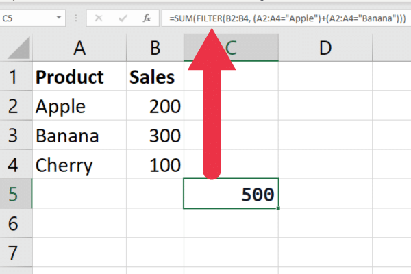
For example, the following formula works on the example data to find matches for two of the three items in the first column and sum their corresponding values in the second column.
=SUM(FILTER(B2:B4, (A2:A4=”Apple”)+(A2:A4=”Banana”)))
This picture shows how many rows are matched and the sum of the different values:
5. Helper Columns
You can use a helper column to join multiple fields together within a function like VLOOKUP.
Suppose you are working with first and last names in a separate sheet. You can concatenate them in a helper column that is referenced within the final formula.
6. Dynamic Arrays
As you’ve learned in earlier examples, Microsoft 365 users can take advantage of dynamic arrays for multiple value lookup in Excel.
Dynamic arrays allow you to return multiple values from a single formula, making it easier to lookup large amounts of data.
7. Power Query
Power Query is a powerful tool in Excel that can be used to return values based on multiple criteria.
For example, this video finds messy data in a spreadsheet and cleans it up.
Final Thoughts
That wraps up our deep dive into the art of looking up multiple values in Excel! Once you’ve mastered the VLOOKUP, INDEX, MATCH, and array formulas, you’ll find yourself breezing through complex data sets like a hot knife through butter.
The key is to understand the syntax and the logic behind each formula. Keep in mind that these formulas can be complex, so it’s important to take your time and test your formulas thoroughly before relying on them for important data analysis.
Excel is a powerful tool, but it’s only as good as the user. So keep honing those skills, keep experimenting, and you’ll soon be the master of multi-value lookups. Until next time, keep crunching those numbers and making Excel do the hard work for you!


