
When working with large datasets in Excel, it’s common to have multiple worksheets containing similar data. Comparing these sheets for duplicate records can be quite a challenge, especially when the data is scattered across various columns and rows.
The most common methods to find duplicates in two Excel sheets are to use:
VLOOKUP, COUNTIF, or EXACT functions
Conditional formatting
Power Query
External tools and add-ins
Visual checks for duplicates
This article walks step-by-step through these five methods to pinpoint and handle duplicates across multiple worksheets. By the end, you’ll see just how easy it to manage duplicate values.

Let’s get started!
Sample Worksheets And Data
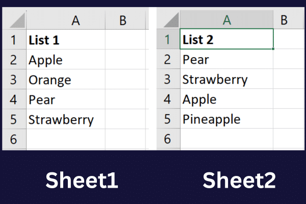
To follow the examples in this article, create a new Excel workbook with this data in column A of the first sheet:
Apple
Orange
Pear
Strawberry
Put this data into column A of the second sheet:
Pear
Strawberry
Apple
Pineapple
Your worksheets look like this:
Once you have your worksheets set up, we can now go over the different ways to find duplicates in two sheets, starting with the VLOOKUP, COUNTIF, and EXACT functions.
Let’s go!

1. Using VLOOKUP, COUNTIF, or EXACT Functions to Find Duplicates
Excel has three built-in functions that can make finding duplicates a breeze: VLOOKUP, COUNTIF, and EXACT.
These functions are designed to help you find, count, and compare data within your spreadsheets, making them ideal tools for finding duplicate entries.
Each function serves a unique purpose and understanding how to use them can significantly streamline your data analysis process.
In the following sections, we will explore how to use the VLOOKUP, COUNTIF, and EXACT functions to effectively identify duplicates in your Excel worksheets.
A. How Do You Use the VLOOKUP Function to Find Duplicates in Two Sheets?
VLOOKUP stands for Vertical Lookup. You use this function to find duplicate values between two columns. This is the syntax:
=VLOOKUP(lookup_value, table_array, col_index_num, [range_lookup])
lookup_value: The value you want to search for in the first column of the table_array.
table_array: The range of cells containing the data you want to search in.
col_index_num: The column number in the table_array you want to return the value from.
range_lookup: Optional. It’s either TRUE (approximate match) or FALSE (exact match). Default is TRUE.
To use the function across two worksheets in an Excel file, you need to know how to reference a separate sheet in a formula. To do so, type the sheet name followed by the exclamation mark (!) and your cell or cell range.
For example, this references cells A2 to A5 in sheet 2 of the same workbook: Sheet 2!$A$2:$A$5.
To use the VLOOKUP function in your sample spreadsheet, follow these steps:
Select cell B2 to display the first comparison result.
Type this formula: =VLOOKUP(A2,Sheet2!$A$2:$A$5, 1, FALSE).
Press Enter to display the comparison result.
Fill down the formula to compare the values for the rest of the rows in the first sheet.
The results will look like the picture below:
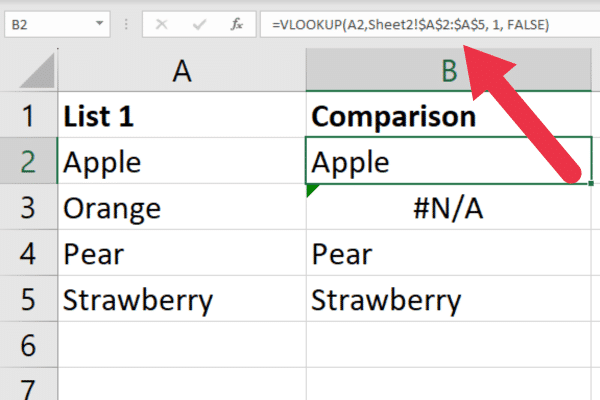
You can tidy up the display by showing a user-friendly message instead of an error when a duplicate is not found.
For example, this formula will display “Yes” or “No” for found and not found values respectively:
=IF(ISNA(VLOOKUP(A2, Sheet 2!$A$2:$A$5, 1, FALSE)), “No”, “Yes”)
There are more examples of this function in our article on using VLOOKUP to compare two columns.
What if You’re Handling Different Workbooks?
If your worksheets are in separate workbooks, the function usage is the same with two Excel files. However, referencing the second worksheet is a little more complex.

You need to:
Enclose the name of the Excel workbook in brackets
Follow with the name of the worksheet
Enclose the workbook and worksheet in quotation marks.
For example, if the cells are in a sheet named Sheet2 in a workbook named “WB 2.xlsx”, the format will look like this:
‘[WB 2.xlsx]Sheet2’!$A$2:$A$5
Before you enter the formula, close the second workbook. Otherwise, you will get an error.
B. How Do You Use the COUNTIF Function to Find Duplicates Across Worksheets?
The COUNTIF function in Excel is used to count the number of cells within a specified range that meet a given criteria.
To compare multiple sheets, you can count the number of cells in the second worksheet that matches a cell in the first worksheet.
This is the syntax of the function:
=COUNTIF(range, criteria)
Range: the range of cells that you want to count based on the specified criteria.
Criteria: the condition that must be met for a cell to be counted.
To use the function with the sample data, follow these steps:
Select cell B2 to display the first comparison result.
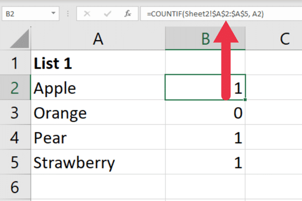
Type this formula: =COUNTIF(Sheet2!$A$2:$A$5, A2)
Press Enter to display the comparison result.
Fill down the formula to compare the values for the rest of the rows in the first sheet.
The function will find one match for some of the cells and none for others. The comparison cell displays the count. Here is the result from the sample data:
The COUNTIF function can be used for other useful tasks such as counting non-blank cells in Excel.
C. How Do You Use the EXACT Function to Find Duplicates Across Worksheets?
The EXACT function in Excel can also be used to look for duplicates within the same cells in two different Excel worksheets. The syntax is:
=EXACT(text1, text2)
text1 is the first text string that you want to compare.
text2 is the second text string that you want to compare.
Follow these steps:
Select cell B2.
Type the formula =EXACT(A2, Sheet2!A2)
Press Enter to display the comparison result. The formula will return TRUE if both values are identical or FALSE otherwise.
Fill down the formula to compare the values for the rest of the rows in the first sheet.
Note that this method doesn’t search for duplicates across a cell range. Instead, you are only looking for matches based on the same cell in a different sheet.
This can be useful with ordered data where you only expect a few exceptions.
The VLOOKUP, COUNTIF, and EXACT functions are useful for finding duplicates, but Excel is a versatile program, and there are other options. In the next section, we look at how you can use conditional formatting to identify duplicates in two sheets.
2. How to Use Conditional Formatting for Duplicate Rows
In this section, you’ll learn how to use conditional formatting to find and highlight duplicate rows in two Excel worksheets.
To create a conditional formatting rule, follow these steps:
Select the range of cells containing the data (A2:A5 in this case).
Click on the “Home” tab in the Excel ribbon.
Click on “Conditional Formatting” in the “Styles” group.
Choose “New Rule” from the drop-down menu.
The next task is to provide a formula for your rule to use. Follow these steps:

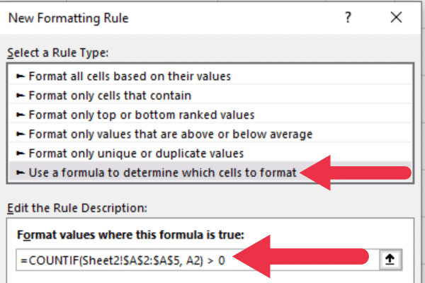
Choose “Use a formula to determine which cells to format” in the dialog box
Enter the following formula: =COUNTIF(Sheet2!$A$2:$A$5, A2) > 0
Finally, you apply the formatting you prefer for duplicate cells.
Click on the Format button to open the Format Cells dialog box.
Choose a format e.g. fill duplicates with a yellow background color.
Click OK.
Your duplicate data is now highlighted in yellow.
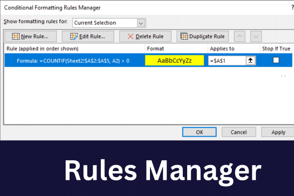
How to Use the Conditional Formatting Rules Manager
Once you’ve created the conditional formatting rule, you can manage it using the Conditional Formatting Rules Manager.
To access the manager:
Go to the Home tab.
Click on Conditional Formatting.
Choose “Manage Rules”.
You will see a list of all conditional formatting rules applied to the selected sheet. You can edit, delete, or change the order of rules by selecting the rule and clicking the appropriate buttons.
To apply the same rule to the other sheet, follow these steps:
Select the range you want to compare in the second sheet.
Go to the Conditional Formatting Rules Manager.
Select the rule, click on Duplicate Rule and then hit Edit Rule.
Replace “Sheet2” with the name of the first sheet to compare.
Now that you’ve applied the conditional formatting rule to both sheets, duplicates will be highlighted according to the formatting you’ve chosen.
Make sure to adjust the range and cell references in the formulas as needed to cover all the data you want to compare.
Conditional formatting might seem a little primitive. If you want finer control, then Power Query may be the answer! In the next section, we cover how you can use Power Query to find duplicates.
3. How to Use Power Query to Find Duplicates Across Worksheets
Power Query is a data transformation and data preparation tool in Microsoft Excel. Identifying the same values is just one of the many analysis tasks you can perform with the tool.
To do so, you should first import the data in the two worksheets into separate tables. Follow these steps within each sheet:
Right-click the cell range.
Choose “Get Data from Table/Range”.
Amend the table name to something appropriate.
After importing both sheets, the first task is to merge the data:
Go to the Data tab.
Click “Get Data”.
Select “Combine Queries”.
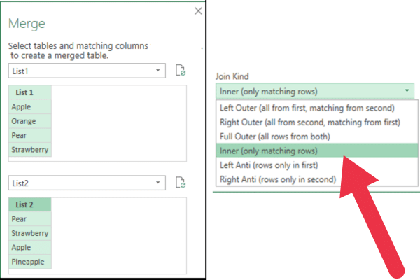
Choose “Merge” and select the two tables.
Click on the two key columns.
Choose “Inner” as the “Join Kind” and click OK.
The Power Query Editor will open with the combined data from both tables in your Excel sheet. You will see two columns, one from each table. Since you are only interested in the duplicate values, you can remove the second column.
You can click “Close & Load” in the Power Query Editor to load the duplicates to a new worksheet.
To explore more aspects of this powerful feature, follow the examples in our article on how to use Power Query in Excel.
Excel also has third-party tools and add-ins that add the ability to seamlessly find duplicates, so let’s take a look at some of those tools in the next section.
4. Tools and Add-Ins to Identify Duplicates Across Worksheets
External tools and add-ins can offer advanced functionality that may not be available in native Excel features. These tools can further streamline the process of comparing sheets for duplicates.
Spreadsheet Compare is a Microsoft tool that allows you to compare two workbooks side-by-side, highlighting differences and easily identifying duplicates. You can download it from the Microsoft website.
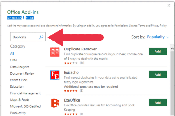
There are several add-ins you can install to automate the process of finding duplicates. One example is “Duplicate Remover”. To install an add-in:
Go to the Insert tab.
Click on “Get Add-In”.
Search for “Duplicate”.
Click “Add” on the tool of your choice.
5. How to Visually Check for Duplicates in Two Sheets
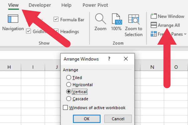
If all else fails, use your eyes! The Arrange Windows dialog box in Excel allows you to view multiple worksheets or workbooks side by side.
While it doesn’t directly find duplicates, it can help you visually compare data across worksheets or workbooks to spot duplicates. Follow these steps:
Click on the “View” tab in the Excel ribbon.
Click on “Arrange All” in the “Window” group.
Choose an arrangement option e.g. “Vertical” or “Horizontal”.
This will display both sheets either side by side or one above the other. Now you can manually compare the data in each sheet to identify duplicates.
You need to scroll through the data and visually inspect each value to find matches.
Note that this method is not efficient for large datasets, as it requires manual comparison. Using the other methods in this article will be more effective for finding duplicates in larger datasets.
And that’s the last of our common methods for finding duplicate values in Excel sheets! In the next section, we’ll give you some tips for preparing your worksheets.
3 Tips for Preparing Your Excel Worksheets
Before you start comparing multiple sheets, make sure you have the columns and rows of your datasets lined up properly.
Ensure that both Excel sheets have the same structure and the same header names. If needed, you can rearrange the columns in both sheets to match each other.
Here are three suggestions to ensure accurate comparisons:
Arrange your data in the same order in both sheets. This makes it easier for Excel functions to work effectively.
Normalize your data by using consistent formatting, capitalization, and data types. This will prevent mismatched entries due to minor differences.
Remove unnecessary blank rows or columns, as they may interfere with the comparison process.
You can assess how much duplication you have in a data set by counting the unique values. This video walks through several methods:
How to Handle Errors and Inconsistencies
Inconsistencies in your data can impact the comparison process. Here are four tips for resolving inconsistencies:
Check for discrepancies in data types, such as mixing text and numerical values in the same column.
Ensure consistent formatting is used for dates, numbers, and other data types.
Examine your data for missing or incorrect entries, and update if necessary.
Standardize abbreviations or inconsistent naming conventions within your data sets.
Final Thoughts
Finding duplicates across two Excel worksheets is an essential task for data management and analysis, ensuring data integrity and accuracy. Excel offers multiple techniques to identify duplicates, each with its own advantages and limitations.
The choice of method depends on the user’s needs, the size and complexity of the dataset, and the desired outcome. For smaller datasets and straightforward comparisons, using VLOOKUP, COUNTIF, or conditional formatting may be sufficient.
For larger datasets or more complex data transformations, Power Query is a powerful and flexible tool that can handle a wide range of data preparation tasks, including finding duplicates.
To wrap it up, comparing Excel sheets for duplicates is a super handy skill to have in your toolbox. With the tricks in this article, you can spot those pesky duplicates and keep your data squeaky clean.
Trust us, as you get better at this, you’ll breeze through your data tasks and impress everyone around you!


