VLOOKUP Between Two Workbooks: Easy Step-By-Step Guide

If you’re working with multiple workbooks in Excel, you may need to use the VLOOKUP function to retrieve data from one workbook to another.

The VLOOKUP function searches for a specific value in a table in a separate workbook and returns a corresponding value from the same row. The syntax must include a fully qualified reference to the second workbook and worksheet name.

Getting the references right can be challenging when you are using the function for the first time. This article uses sample spreadsheets to show you exactly how to input the formulas.

You’ll also learn some enhancements to VLOOKUP and several alternatives to the function.

Let’s get started!

What is VLOOKUP?

Suppose you have a workbook of product sales and a separate workbook with the prices of each product. You want to access the prices from the second workbook and use them in calculations in the first workbook.

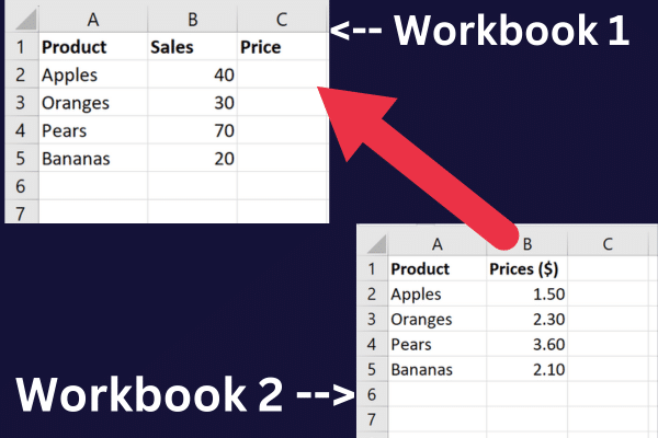
VLOOKUP is one solution for this task. The term stands for “Vertical Lookup.“

It is an in-built function that allows you to search for a specific value in a column and return a corresponding value in another column based on the location.

It can be used with:

• a single spreadsheet

• multiple sheets in the same workbook

• two Excel workbooks

If you don’t have the additional complexity of multiple workbooks, check out this tutorial on comparing two columns in Excel using VLOOKUP.

How to Use VLOOKUP Between Two Workbooks

The VLOOKUP function is especially useful when you need to search for data across multiple worksheets or workbooks.

The three main steps to do so are:

1. Open both workbooks.

2. Enter the VLOOKUP formula in the first Excel workbook.

3. Provide a fully qualified reference to the second workbook.

Sample Data

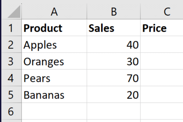
This simple tutorial works through examples based on sample data. To follow along, create a new workbook called “Sales” and enter this data in columns A and B:

• Apples, 40

• Oranges, 30

• Pears, 70

• Bananas, 20

Add a third column to hold the Price information:

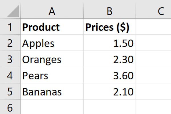
Create a second Excel workbook called “Product” and rename Sheet1 as “Prices”. Enter this data in column A and column B:

• Apples, 1.50

• Oranges, 2.30

• Pears, 3.60

• Bananas, 2.10

The data looks like this:

To calculate the revenue for the sales in the first spreadsheet, we need to look up the price in the second spreadsheet. VLOOKUP to the rescue!

Step 1: Keep Both Workbooks Open

Both workbooks must be open when using the VLOOKUP formula between two workbooks. If the second workbook is closed, the function will return an error.

You can either open them separately or use the “Open” command in Excel to open them both at once. There are two ways to open either workbook:

• Go to the File tab and select “Open”.

• Use the “Ctrl + O” keyboard shortcut.

Once you have both workbooks open, you can switch between them by clicking on the appropriate tab at the bottom of the Excel window.

Step 2: Start Entering the VLOOKUP Formula

Here is the basic syntax of the VLOOKUP function:

=VLOOKUP(lookup_value, table_array, col_index_num, [range_lookup])

• lookup_value: The value you want to look up in the other workbook.

• table_array: The range of cells in the other workbook that contains the data you want to retrieve.

• col_index_num: The column number in the range that contains the data you want to retrieve.

• range_lookup: This last parameter is optional. If you set it to TRUE or omit it, VLOOKUP will look for an approximate match. If you set it to FALSE, VLOOKUP will only look for an exact match.

Let’s say you want to look up the price of apples in the second workbook of our sample data. This is how the formula will break down:

• The lookup_value is in cell A2 of the first workbook.

• The table array is in the cell range A1:B5 of the second workbook.

• The col_index_num is the second column that holds the price.

The most complicated part of the VLOOKUP formula is referencing the second workbook correctly.

Step 3: How to Reference the Second Workbook

To complete the VLOOKUP formula for two workbooks, you’ll need to use a fully qualified reference that includes these details from the second workbook:

• workbook name

• sheet name

• cell range

This ensures that Excel knows exactly where to find the data you’re looking for. The fully qualified reference is used for the table_array argument of the VLOOKUP function.

These are the values for the sample data:

• workbook name: Product.xlsx

• sheet name: Prices

• cell range: $A1:$B5

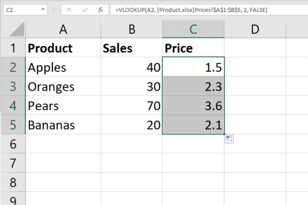
To look up the price for the first item, enter the following formula into cell C2 of the first workbook:

=VLOOKUP(A2, [Product.xlsx]Prices!$A$1:$B$5, 2, FALSE)

This picture shows the function in action in the formula bar for the first cell:

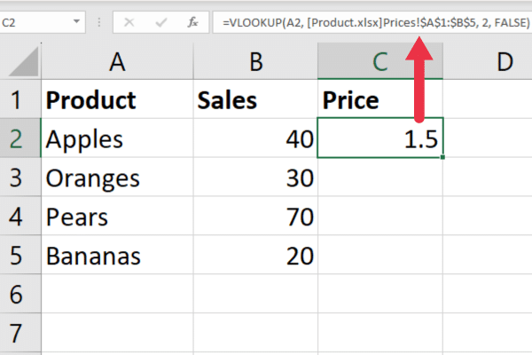
Note that the workbook name is enclosed in square brackets, and the sheet name is followed by an exclamation point.

If the Excel file name contains a space or special characters, then you must enclose the entire workbook and sheet in single quotes.

The formula uses absolute values for the cell range (the $ prefix). This allows you to copy down the formula to the rest of the rows by clicking on the fill handle.

Here are the VLOOKUP results:

And that’s it! You now know how to use VLOOKUP effectively. To help you in case you run into any errors, we’ve compiled three of the most common VLOOKUP errors in the next section.

3 Common VLOOKUP Errors and How to Fix Them

Now that you’ve learned how to use VLOOKUP from another workbook, you may encounter some common errors.

Here are the three most frequent errors and how to fix them.

1. #N/A Error

The #N/A error occurs when the lookup value is not found in the table array. To fix this error, you can try the following:

• Check the spelling of the lookup value.

• Make sure that the lookup value is in the first column of the table array.

• Check that the lookup value is not formatted as text in the two sheets.

• Ensure that the range_lookup argument is set to FALSE to find an exact match.

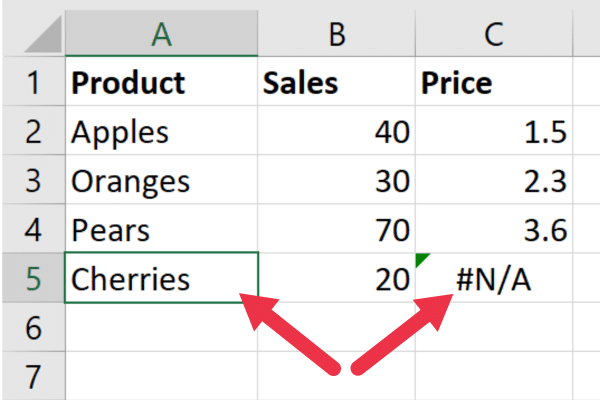
The above example has failed to find a matching value for Cherries in the second workbook.

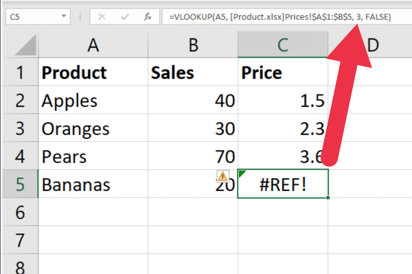
2. #Ref! Column Number Error

The #Ref! Error happens when the col_index_num argument is greater than the number of columns in the table array.

To fix this error, check that the col_index_num argument is less than or equal to the number of columns in the source table.

In the picture below, the col_index_num has been set to 3 but there are only two columns in the reference range.

3. Quotes and Square Brackets Error

The Quotes and Square Brackets Error happens when you perform VLOOKUP with a value containing quotes or square brackets.

To fix this error, you can try the following:

• Use double quotes around the lookup value.

• Use the CHAR(34) function to insert double quotes.

• Use the IFERROR function to return a blank cell if the lookup value contains quotes or square brackets.

Once you’re familiar with these errors, fixing them is straightforward! To further help you become a VLOOKUP pro, we’ve provided four tips for managing different workbooks in the next section.

4 Tips for Managing Different Workbooks

When working with multiple workbooks, it is important to keep track of which workbook contains which data.

Here are our four best tips to keep your sanity:

1. Use naming conventions to help you remember which Excel spreadsheets contain which data.

2. Use absolute references in your formulas to ensure that the lookup range references the correct cells even if you move or copy the formula to another location or Excel sheet.

3. Use the IFERROR function to handle any #N/A errors that may occur if the lookup values are not found in the source data.

4. Consider locking the cells in the reference workbook so that they can’t be overwritten.

How to Update Data Automatically

When working with multiple Excel files, it can be time-consuming to update the data manually.

If you want your VLOOKUP formula to update automatically when you add or remove data from the other workbooks, you can use the INDIRECT function.

Here’s how:

• In the VLOOKUP formula, replace the table array argument with the INDIRECT function.

• In the INDIRECT function, use a reference to the cell that contains the table array in the other workbook.

To achieve this with our sample workbooks, follow these steps.

1. Use one cell in column D to enter the reference to the “Product” workbook’s “Prices” sheet and the cell range A1:B5 like this: [Product.xlsx]Prices!A:B

2. In cell C2 of the “Sales” workbook, use this formula: =VLOOKUP(A2, INDIRECT($D$1), 2, FALSE)

3. Copy the formula down (the absolute references ensure that the cell with the spreadsheet is preserved).

These actions ensure that changes in the original sheet get automatically updated in the connected cells.

This picture shows the INDIRECT function combined with VLOOKUP:

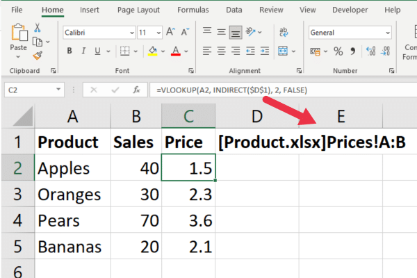
Note that this example uses the range “A:B” to reference the two columns. This means that when you add more products and prices, the formula will continue to work in the current workbook.

Now that you’ve gotten a taste of VLOOKUP’s power, let’s take a look at some advanced uses of the function in the section!

Advanced Uses of the VLOOKUP Function

The examples in this article return a single match for each lookup value. If you want to work with multiple matches from a different workbook, you can use an array formula instead.

You can also combine VLOOKUP with other functions. For example, you can embed it within an IF function for additional complex analysis.

Complex analysis includes techniques like chi-square tests and paired samples T-tests. Here’s an example of using the chi-square test in Excel:

Advanced users take advantage of VLOOKUP to compare data sets and identify mismatches. You will find other ways in this article on finding discrepancies in Excel.

But what if you don’t want to use VLOOKUP for whatever reason? You’re in luck! There are some alternatives, which is what we’ll cover in the next section.

2 Main Alternatives to VLOOKUP

When it comes to looking up values in different sheets, VLOOKUP is often the go-to function. However, there are some alternatives that can be useful in certain situations.

The two most common are:

• INDEX MATCH

• XLOOKUP

1. INDEX MATCH

INDEX and MATCH is a powerful combination of two functions that can be used to look up values in a table. Unlike VLOOKUP, which requires the lookup value to be in the leftmost column of the table, INDEX MATCH can look up values in any column.

Here’s how it works:

1. The INDEX function returns a value from a specified range based on a row and column number.

2. The MATCH function returns the position of a lookup value in a specified range.

To use INDEX MATCH, you need to specify the range you want to search, the row where you want to find the lookup value, and the column where you want to return the result.

Here’s an example formula:

=INDEX(TableRange,MATCH(LookupValue,LookupRange,0),ColumnIndex)

To use this with the sample spreadsheets, this is the formula:

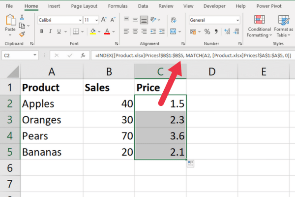
=INDEX([Product.xlsx]Prices!$B$1:$B$5, MATCH(A2, [Product.xlsx]Prices!$A$1:$A$5, 0))

This breaks down as:

• The MATCH function searches for the value in cell A2 (product name) within the range A1:A5 in the “Prices” sheet of the “Product” workbook.

• The INDEX function returns a value from the range B1:B5 in the “Prices” sheet of the “Product” workbook, based on the row number provided by the MATCH function.

This picture shows the formula in action:

2. XLOOKUP

XLOOKUP is a newer function that was introduced in Excel 365. It is similar to VLOOKUP, but with some additional features.

One of the biggest advantages of XLOOKUP is that it can look up values to the left of the lookup column.

Here’s how it works:

1. The XLOOKUP function returns a value from a specified range based on a lookup value.

2. You can specify whether you want an exact match or an approximate match.

3. You can also specify what to return if no match is found.

To use XLOOKUP, you need to specify the lookup value, the range you want to search, and the column where you want to return the result.

Here’s an example formula:

=XLOOKUP(LookupValue,LookupRange,ReturnRange,”Not Found”,0)

To use this with the sample spreadsheets, this is the formula:

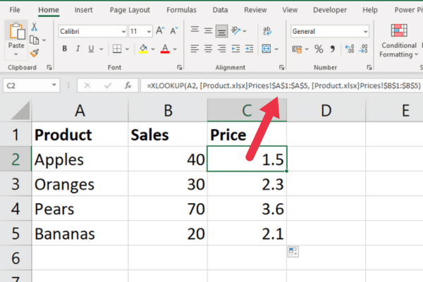
=XLOOKUP(A2, [Product.xlsx]Prices!$A$1:$A$5, [Product.xlsx]Prices!$B$1:$B$5)

This breaks down as:

• A2: The value you want to look up (product name).

• [Product.xlsx]Prices!$A$1:$A$5: The range where you want to search for the lookup value (product names in the “Prices” sheet of the “Product” workbook).

• [Product.xlsx]Prices!$B$1:$B$5: The range that contains the return values (prices in the “Prices” sheet of the “Product” workbook).

This is the formula in action:

How to Use VLOOKUP Across Multiple Sheets

If you need to perform a VLOOKUP between two workbooks, you may also need to use VLOOKUP across multiple sheets.

Fortunately, the process for doing so is very similar to performing a VLOOKUP between two workbooks.

There are four steps.

Step 1: Identify the Components

Rather than including the table array as you would for one sheet, you will need to include the sheet name as well.

For example, if you want to search for a value in the range A2:B6 on the Jan sheet in the Sales_reports.xlsx workbook, your formula would look like this:

=VLOOKUP(A2,[Sales_reports.xlsx]Jan!$A$2:$B$6,2,FALSE)

Step 2: Set Up Your Data

Make sure that your data is organized in a way that makes it easy to reference across multiple sheets.

You may want to consider creating different tabs for specific reference data.

Step 3: Use the VLOOKUP Function

Once your data is set up, you can use the VLOOKUP function to search for and retrieve data from other sheets.

Just make sure to include the sheet name in your formula, as shown above.

(Optional) Step 4: Troubleshoot #N/A Errors

If you encounter #N/A errors when using VLOOKUP across multiple sheets, double-check your formula to make sure that you have correctly referenced all of the necessary sheets and ranges.

You may also want to check that you are performing an exact match, rather than a range lookup.

Final Thoughts

You’ve learned how to use VLOOKUP to search and retrieve data across two spreadsheets. This versatile function makes it easy to look up values in one workbook based on corresponding values in another.

The VLOOKUP function’s power extends well beyond single worksheets, reaching across different workbooks to link and analyze data.

Mastering this function is a significant step towards becoming proficient in Excel, as it opens up new possibilities for managing and interpreting your data.

By incorporating functions like INDIRECT, INDEX-MATCH, or XLOOKUP, you can further enhance the flexibility and effectiveness of your data lookups.

Keep practicing and exploring the vast capabilities of Excel; this is just the tip of the iceberg. Happy data hunting!