
When working with large datasets in Microsoft Excel, encountering discrepancies in the data is inevitable. Identifying and fixing these inconsistencies is critical for ensuring accurate reporting and analysis.
The good news? Excel comes with a variety of tools and techniques to help you find and resolve these issues. In this article, you will learn about some of the most effective methods. This includes filtering, conditional formatting, and using advanced formulas.
By incorporating these techniques into your everyday workflow, you’ll become more efficient in managing and analyzing your data. Ultimately leading to better decision-making and improved outcomes for your projects.

Understanding Discrepancies in Excel
Discrepancies in rows and columns can result from human input errors, duplicate entries, or irregularities in data formatting.
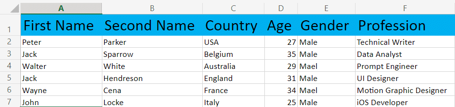
Take a look at the following data. You’ll notice that the Gender of Walter White and Wayne Cena is misspelled – Mael instead of Male. Indeed, it’s straightforward to notice and fix the errors in this scenario. But that isn’t the case with spreadsheets containing thousands of rows & cols.
To find and manage these discrepancies, you can use the following Excel features:
- Filters: Apply filters to specific columns to view unique values and quickly spot inconsistent data.
- Conditional Formatting: Use formatting rules to highlight cells that meet specific criteria or mismatched data between columns.
- Advanced Excel Functions: Utilize functions such as MATCH and VLOOKUP to compare data sets and identify discrepancies between them.
By understanding how to use these features in Excel, you can efficiently spot and rectify discrepancies in your data sets.
5 Ways to Find Discrepancies in Excel
There are 5 main ways we like to tackle discrepancies in Excel:
- Manual Review
- Filtering
- Conditional Formatting
- Advanced Excel Functions
- Excel Add-ins
Let’s run through each of them so that you can work out the best way that suits you.

#1 – Finding Discrepancies via Manual Review in Excel
When working with Excel, a manual review can be a helpful method for identifying discrepancies in your data. This process requires careful examination of the data sets to spot any inconsistencies or errors.
Here are some steps you can follow to perform a manual review:
- Begin by clearly understanding the data sets you are working with. Make yourself familiar with the rows, columns, and formatting.
- Scroll through the data and pay close attention to the information presented in each cell. You can use tools like cell highlighting with fill color, text formatting, or conditional formatting to make data easier to read.
- Compare one row against another or one column against another. Look for mismatched information, duplicate entries, etc. that may cause inaccuracies in your Excel sheets.
- As you identify discrepancies, create a list or use comments to document them. Later on, these can serve as important references for correcting the issues.
When manually reviewing data for discrepancies in an Excel spreadsheet, patience is the key. This process is time-consuming. But it’s a good starting point to identify potential errors.

#2 – Using Filter in Excel to Detect & Fix Inconsistent Data
One of the easiest ways to detect inconsistent data is by using Excel’s Filter.
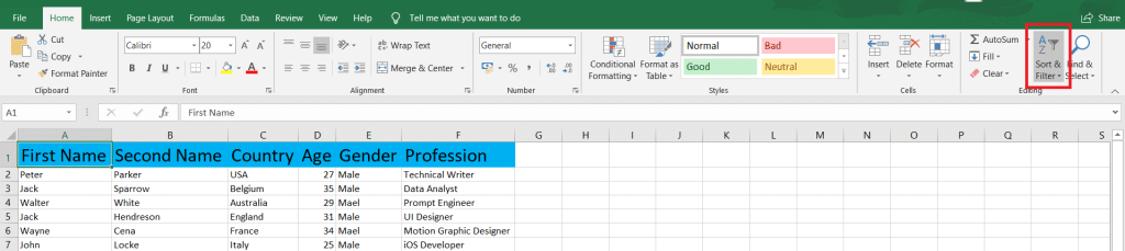
With Filter, we’ll isolate the incorrect data in the Gender column in the following data set:
1. Select the Sort & Filter in the Home tab.
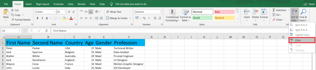
2. Choose Filter – ensure your cursor is in the range of the data.
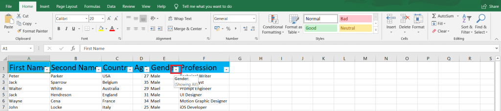
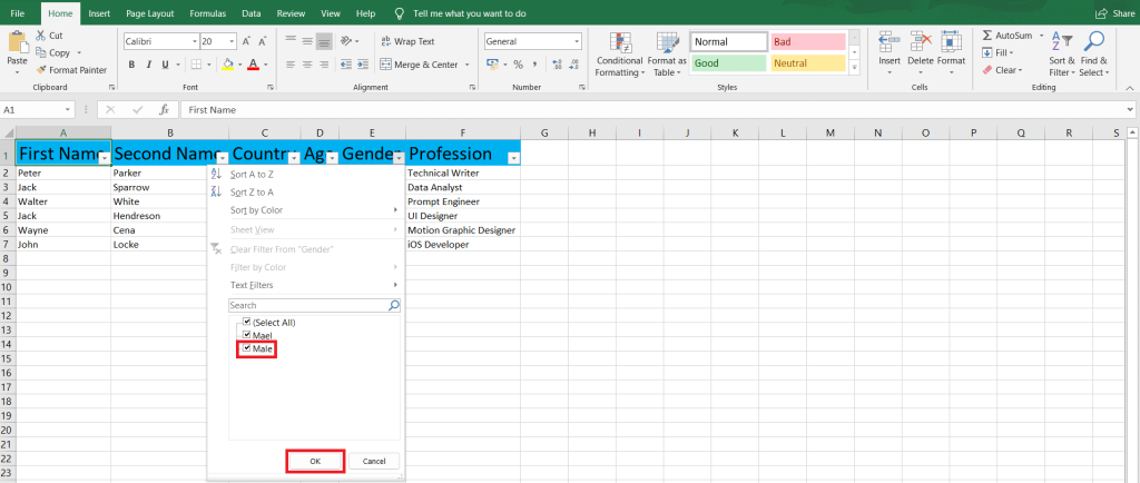
3. Click the drop-down list arrow on the column with inconsistent data.
4. Now, de-select all the correct matching data. In our case, it’s Male. Then, click OK to save changes.
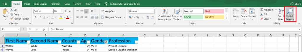
5. Your Excel worksheet will now only show rows with incorrect values. To fix them, click Find & Select in the Home tab.
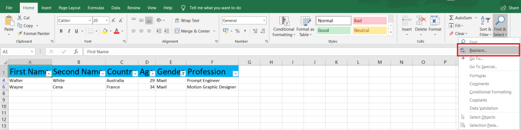
6. Click Replace when the drop-down list appears.
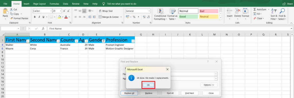
7. Type the incorrect value in Find what and the correct one in Replace with. Then, click Replace All.
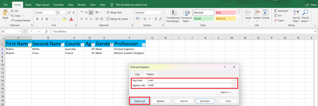
8. A dialog box will appear confirming the changes. Click OK to continue.
3# – Highlighting Discrepancies with Conditional Formatting
Another way to identify column and row differences is by using conditional formatting.
You can access rules like Highlight Cells, Top/Bottom, Data Bars, Color Scales & Iron Sets. Moreover, you can create a new rule and manage or clear previous rules.

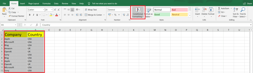
We’ll use a sample table to show you the power of conditional formatting:
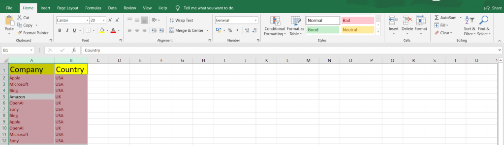
1. Select your table or preferred rows and columns. We are choosing Column A (Company) and Column B (Country). Then, select Conditional Formatting on the Home tab.
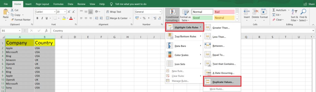
2. Select a rule type and then the rule. We are picking Highlight Cell Rules and Duplicate Values…
3. Now, we have to select whether to highlight Duplicate or Unique values and the Fill Color & Font to format cells. Once done, click OK.
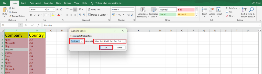
4. All the duplicate values are now highlighted with Light Red Fill with Dark Red Text.
#4 – Finding Discrepancies with Advanced Excel Functions
IF and IS Functions
To compare cells and identify differences, you can utilize IF and IS functions.
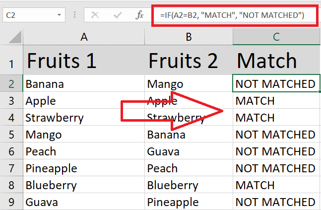
For example, we have used the formula =IF(A2=B2,"MATCH","NOT MATCHED") to compare cells A2 and B2. And we have dragged the formula to apply it to other cells. So, identical cells are returning MATCH otherwise NOT MATCHED.
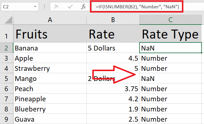
You can combine IF with IS functions like ISNUMBER or ISTEXT to check for specific data types. For example, the formula =IF(ISNUMBER(B2), "Number", "NaN") will return Number in column c if B2 is numeric and NaN otherwise.
VLOOKUP, HLOOKUP & XLOOKUP
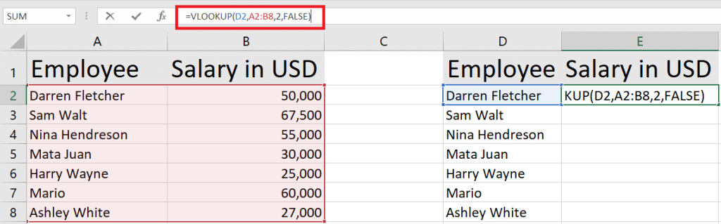
VLOOKUP (Vertical) and HLOOKUP (Horizontal) functions are useful when comparing values in different columns or rows of two tables. To do it, use the following formula: =VLOOKUP(lookup_value, table_array, col_index_num, [range_lookup]) or =HLOOKUP(lookup_value, table_array, row_index_num, [range_lookup]).
Replace lookup_value with the value you want to find in the other table, table_array with the range of cells in the second table, col_index_num or row_index_num with the index number of the column or row you want to return a value from, and [range_lookup] with FALSE for exact matches or TRUE for an approximate match.
In the following tutorial, we are using the VLOOKUP function on Column E to compare Employee Names in Column A and Column D to pull off their Salaries from Column B if a match is found.
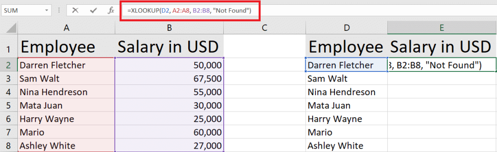
XLOOKUP is a refreshed version of VLOOKUP and HLOOKUP available on Excel 2021 and Excel 365. To XLOOKUP formula is: =XLOOKUP(lookup_value, lookup_array, return_array,[if_not_found]).
Substitute lookup_value with the value you want to find in the other table, lookup_array with the range of cells to search in the second table, return_array with the array you want to return a value from, and [if_nout_found] with a text value if no matching values are found.
Here’s a quick sample of XLOOKUP with the same tables:
MATCH
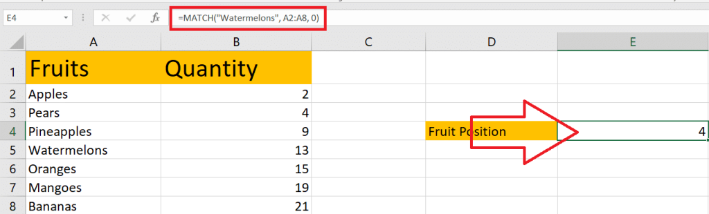
The MATCH function can also be used to compare two lists for discrepancies.
The MATCH function, =MATCH(lookup_value, lookup_array, [match_type]), searches for a specified item in a range and returns the relative position of the item within that range.
Here, we are finding the position of Watermelons in the array A2:A8 using MATCH. We are using match_type as 0 to find the first value that’s exactly equal to the lookup_value.
#5 – Using Excel Add-ins for Discrepancy Detection
Excel offers various add-ins and built-in tools that can help you detect and analyze discrepancies more efficiently. In this section, we will discuss some of those useful add-ins.
First, consider using the Spreadsheet Inquire add-in. This can help you compare two workbooks and highlight differences cell by cell. To enable the Spreadsheet Inquire add-in:
1. Click the File tab.

2. Select Options, and then click the Add-Ins category.
3. In the Manage box, select COM Add-ins and click Go.
4. Check the Spreadsheet Inquire box and click OK.
5. Once enabled, navigate to the Inquire tab to use the Compare Files command.
Another useful tool for discrepancy detection is the Analysis ToolPak. This add-in provides advanced statistical functions and data analysis tools, which can be useful when analyzing discrepancies.
To enable the Analysis ToolPak, follow the same steps as enabling the Spreadsheet Inquire add-in. But select Excel Add-ins in the Manage box and check the Analysis ToolPak box.
In summary, Excel offers various add-ins to help you detect and handle discrepancies in your data. You can improve your data accuracy by familiarizing yourself with these tools and formulas.
How Can Can You Creat Data Validation Rules to Prevent Discrepancies?
To create data validation rules in Excel that can help prevent discrepancies, follow these steps:
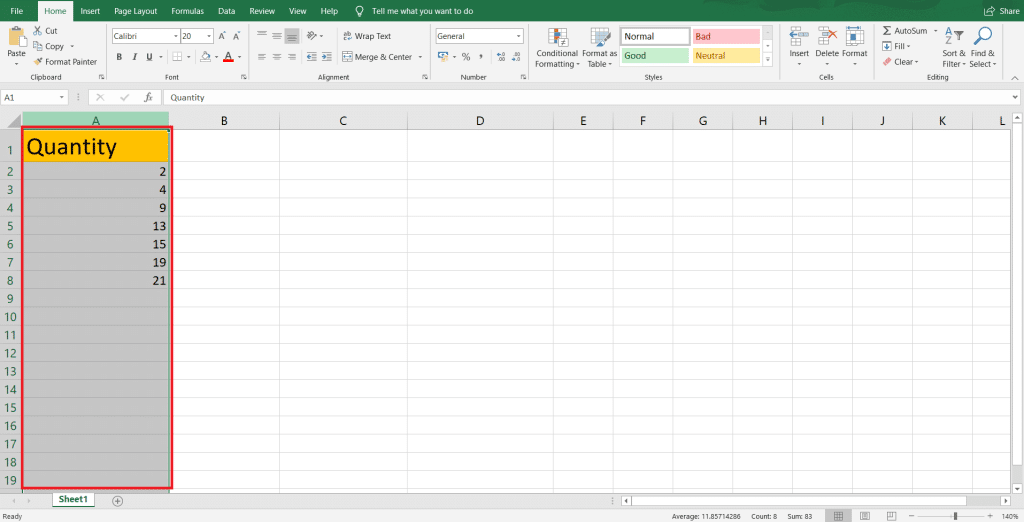
1. Select the cells you want to restrict. This can be a single cell, a range of cells, or an entire column.
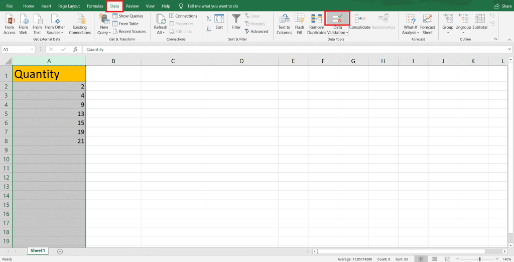
2. Go to the Data tab in the toolbar, and click the Data Validation button (marked by two horizontal boxes, a green checkmark, and a red crossed circle).
3. In the Data Validation window, ensure you are on the Settings tab. Here, you will have the opportunity to define your validation criteria based on your needs.
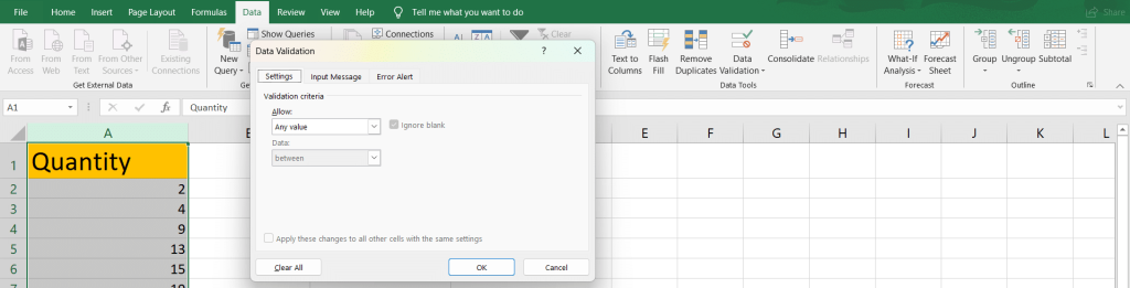
There are various types of validation criteria available in Excel, some of which include:
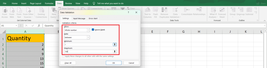
- Whole number – allows only whole numbers within a specified range.
- Decimal – permits only decimal numbers within a specified range.
- List – restricts input to a predefined list of acceptable values.
- Date – requires dates within a specific date range.
- Time – accepts only times within a particular time range.
- Text length – enforces constraints on the length of the text entered.
- Custom – enables you to create custom validation rules using Excel formulas.
After selecting the appropriate validation criteria, specify the parameters as needed. For instance, if you chose Whole Number, you would have to set the Minimum and Maximum with a Data range validator like between, equal to, less than, etc.
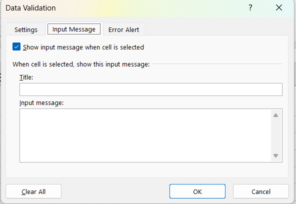
In addition to the validation criteria, you can also set up custom error messages and input hints to help users understand and adhere to your validation rules. To do this, switch to the Input Message and Error Alert tabs to enter your desired messages.
By implementing data validation rules, you significantly reduce the likelihood of data inconsistencies and improve the overall accuracy of your Excel worksheets.
Our Final Word
In this article, you’ve learned various methods to find and address discrepancies in your Excel data. Let’s recap those key strategies:
- Using Filter drop-downs in columns to identify unique values and inconsistent data.
- Employing Conditional Formatting in selected cells to highlight discrepancies using a bunch of rule templates.
- Applying advanced Excel functions like MATCH, VLOOKUP, XLOOKUP, etc. functions to cross-check data in two lists or tables.
- Using Excel add-ins to detect discrepancies.
- Setting up Data validation rules to prevent errors in data
With these techniques in your Excel skillset, your data will be more accurate and trustworthy.
Remember to practice these methods regularly to become more efficient at detecting discrepancies in your spreadsheets.
Keep refining your skills by signing up for our Free Training, and continue exploring new features and functionalities to become even more proficient in Excel.


