
When working with large datasets in Excel, you may need to compare two columns to find similarities or differences.
VLOOKUP is a powerful function that allows you to search for matching data between two columns. The function allows you to search for values in one column that appear in another.
This article shows you how to compare two columns using VLOOKUP, so you can efficiently analyze your data.

Fundamentals of Vlookup Function
Suppose you have a spreadsheet with two lists of items in column A and column B. You want to find the items in List 1 that also appear in List 2.
You can imagine that working manually through lists of thousands of items would be hugely time-consuming. Thankfully, Excel brings VLOOKUP to the rescue!
The term VLOOKUP stands for Vertical Lookup. The function will compare two columns, finds matches between them, and returns the associated values.
Vlookup Function
Here’s a basic syntax of the VLOOKUP function:
=VLOOKUP(lookup_value, table_array, col_index_num, [range_lookup])
This is a breakdown of the elements:

lookup_value: the value you want to search for in the first column of the table_array.
table_array: the range of cells containing the data you want to search in.
col_index_num: the column number in the table_array you want to return the value from.
range_lookup: Optional. It’s either TRUE (approximate match) or FALSE (exact match). The default is TRUE.
Preparing Your Data for VLOOKUP
Before using VLOOKUP to compare two columns in Excel, you need to prepare your data.
Create two separate columns in your worksheet where you want to compare the values. This article uses Column A and Column B for our examples.
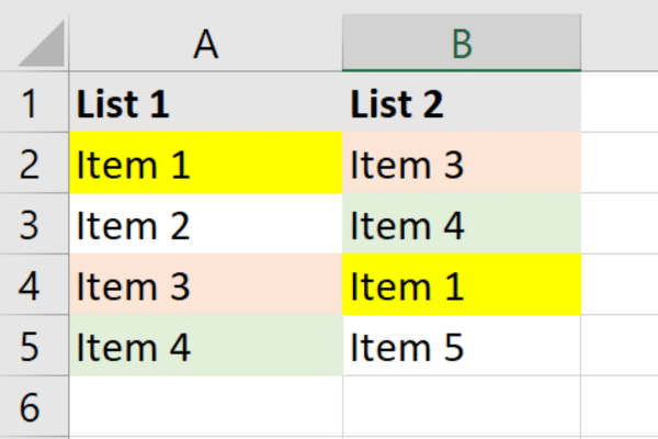
Here is the sample data used in this article:
This is the sample table with header to be added to the section titled “Preparing Your Data for VLOOKUP”:
List 1 List 2
Item 1 Item 3
Item 2 Item 4
Item 3 Item 1
Item 4 Item 5
Formatting the data
It’s important to ensure that the data in both columns are formatted similarly. VLOOKUP is case-sensitive,which means that capitals and lower-case characters matter.
Matching errors may occur in the final result if the formatting is inconsistent.
It’s also a good idea to remove any duplicate values or blank cells to minimize the risk of errors.
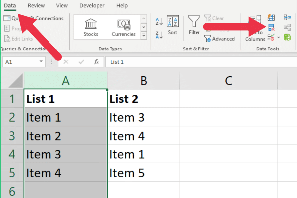
To remove duplicate values:
Select the column.
Go to the Data tab in the top ribbon.
Click on Remove Duplicates in the Data Tools section.
The button can be a little hard to see. This picture will help you:
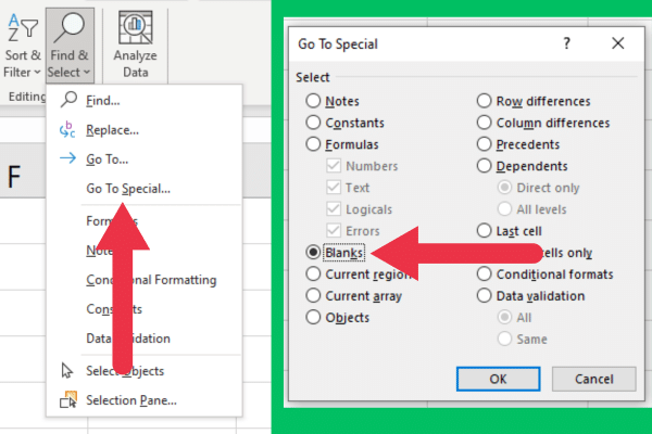
To remove blank cells:
Select the column.
Go to the Home tab in the top ribbon.
Expand the “Find & Select” menu.
Choose “Go to Special”.
Select “Blanks” from the options.
Click on “Delete” in the Cells section.
How To Use VLOOKUP To Compare Two Columns
Once data is prepared, you can write the VLOOKUP formula to compare two columns in Excel and identify matches. Follow these steps:
Select a cell in a new column where you want to display the comparison results (e.g., cell C2).
Type the following formula: =VLOOKUP(A2, B:B, 1, FALSE))
Press Enter to apply the formula.
In case of a matching value, the value will be displayed in the same row of the result column (e.g., Column C).
Drag the formula down from C2 to copy it over as many cells as you need.
If you’re using our sample data, put your comparison results in the third column. The formula will find three matches out of the four items in List 1.
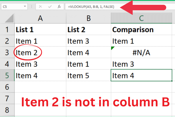
Notice that Item 2 is showing as #N/A. Excel is telling us that the match is not applicable i.e. it could not be found.
That is correct and is useful information about missing values. However, some Excel users may think that there is some data issue or function error.

It’s good practice to show a different indication that no match was found. That could simply be a blank.
To do so, combine the VLOOKUP function with the IFNA function like this:
=IFNA(VLOOKUP(A1, B:B, 1, FALSE), “”)
The IFNA function detects the #N/A error and replaces the output with an empty space (“”). You can also use the ISNA function or have additional logic with the IF function.
Handling other errors
VLOOKUP can sometimes generate other errors in your comparison results. The #REF! Error in Excel is a genuine problem with your data.
It usually occurs when your specified range is incorrect. Our example has referenced the entire column, but you can also use vertical cell ranges.
Make sure the search range you are referring to covers all the values you want to compare.
Alternatives to VLOOKUP for Column Comparison
There are two main alternative lookup functions when comparing two columns in Excel to find matches.
1. Using Index and Match Functions
Instead of using VLOOKUP, you can compare two columns in Excel by combining the INDEX and MATCH functions.
This method provides a more flexible way to look up data and is particularly useful when working with non-adjacent columns or when the column index may change.
This is the syntax to put in the result column:
=INDEX(return_range, MATCH(lookup_value, lookup_range, 0))
Return_range: the range of cells that contain the data you want to return.
Lookup_value: the value you want to search for within the lookup range.
Lookup_range: the range of cells within which you want to find the lookup value.
Using the same data in the previous examples, we replace the VLOOKUP formula as follows:
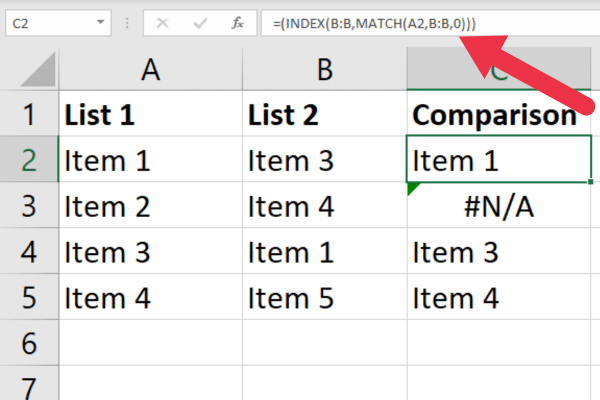
=(INDEX(B:B, MATCH(A2, B:B, 0)))
The MATCH function returns the relative position of the lookup value within the lookup range, and the INDEX function returns the corresponding value from the return range.
The results on the same data will be the same as the VLOOKUP we used earlier. This picture shows the functions in use:
You can also replace the #N/A error with a custom message. Here is an example of using the IFERROR function.
=IFERROR(INDEX(B:B, MATCH(A2, B:B, 0)), “Not Found”)
2. Employing XLOOKUP in Excel
For users with Excel 365 or Excel 2019, XLOOKUP is an alternative logical test to VLOOKUP for finding common values in two columns.
XLOOKUP provides several advantages. You can use it to search data both horizontally and vertically, work with non-adjacent columns, and specify custom values for errors.

The syntax of XLOOKUP is:
=XLOOKUP(lookup_value, lookup_range, return_range, [if_not_found], [match_mode], [search_mode])
lookup_value: the value you want to search for within the lookup range.
lookup_range: the range of cells within which you want to find the lookup value.
return_range: the range of cells that contain the data you want to return.
Add custom error values, match mode, and search mode parameters as needed.
XLOOKUP will find the lookup value within the lookup range and return the corresponding value from the return range.
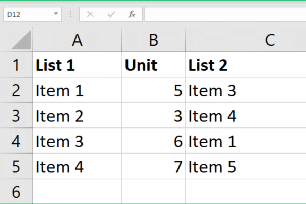
The formula is particularly useful when you have two lists embedded in data sets of multiple columns. In our previous examples, the lists have been in the first column and second column, but your sheet may have more data than that.
Here is an example with two lists in the first and third column of a spreadsheet:
The XLOOKUP formula looks like this:
=XLOOKUP(A2,C:C,C:C,””)
This picture shows the result with the comparison in column D. The first value is present but the second is missing.
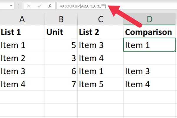
Note that I have no extra error formulas but the missing value is displayed as a blank. That’s because I’m using the fourth parameter which is a custom error value. In this case, it’s a blank string.
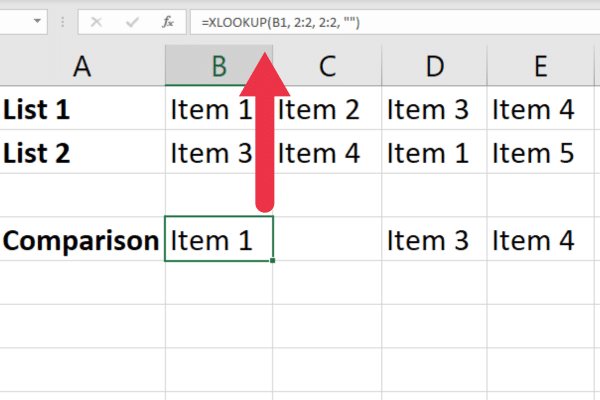
As a bonus, I’ll show you how to use XLOOKUP to compare across rows. If you have two lists that are in row 1 and row 2, the simplest use of the formula looks like this:
=XLOOKUP(B1, 2:2, 2:2, “”)
This picture shows the results on the two rows.
With its improved functionality and flexibility, XLOOKUP is an excellent alternative to VLOOKUP for comparing lists in Excel to determine if matches are present.
Five Tips to Improve VLOOKUP Performance
Optimizing your VLOOKUP function can help you avoid long waiting times and improve the overall responsiveness of your Excel worksheet.
Here are six tips and tricks you can apply to improve the performance of your VLOOKUP in Excel.
1. Limit your lookup range
I used entire columns in the examples to make them simple. If you are working with a large amount of data, you should avoid doing so. Using full columns can slow down Excel’s calculation process.
Instead, try to use the exact range required for your data (e.g., A1:A100). This reduces the number of cells that your VLOOKUP function needs to evaluate.
2. Use absolute references
When specifying a data range (e.g. the cells from B2 to B5), use absolute references. This ensures that the formula is consistent and data exists when you copy it across multiple cells.
Here is an example:
=VLOOKUP(A2, $B$2:$B$5, 1, FALSE)
3. Sort your data
If you know that the data in the lookup column is sorted in ascending order, you can use VLOOKUP with a TRUE or 1 for the ‘range_lookup’ argument.
This will cause Excel to perform an approximate match, which is faster than an exact match across all the cells. However, be cautious when using this option, as an incorrect sort might lead to incorrect results.
4. Use a double VLOOKUP
You can use two VLOOKUP functions to speed up the search process in Excel.
The first VLOOKUP will determine if the lookup value exists by setting the ‘col_index_num’ to 1 and the ‘range_lookup’ to TRUE.
If it returns TRUE, a second VLOOKUP retrieves the desired value with the ‘range_lookup’ set to TRUE.
5. Use conditional formatting
You can use conditional formatting in your Excel worksheet to highlight matching or missing values in the specified column. You can also apply colors to unique values. This makes your data easier to read.
You will find the conditional formatting menu in the styles group on the Home tab.
Advanced Uses For VLOOKUP
Paired samples T-tests are used to compare the means of two related samples. This video shows their use in Excel.
If you have additional data or variables that you need to reference during your analysis, you can use VLOOKUP to retrieve the necessary values from another table or worksheet.
For example, you may use VLOOKUP to retrieve demographic information or treatment conditions for each paired observation in your dataset.
Our Final Word
By now, you have a solid understanding of using VLOOKUP. This powerful function allows you to quickly identify differences and matching values between two lists, making data analysis more efficient and accurate.
You also saw examples of other lookup and reference functions, such as XLOOKUP, INDEX, and MATCH. Adding these elements to your skills will further strengthen your data analysis capabilities.
Keep practicing and refining your VLOOKUP skills, and you’ll soon become an expert at comparing columns in Excel, saving time and boosting your productivity.


