
There are times when you want to lock specific cells in an Excel worksheet to protect them from accidental editing.
By locking cells, you can ensure that important data remains unchanged while still allowing other users to make changes to other parts of the spreadsheet.
This article shows you how to lock cells in Excel in four simple steps:

Unlock all cells in the worksheet.
Select the cells you want to lock.
Use the Format Cells dialog box to lock the selected cells.
Go to the Review tab in the Excel ribbon and protect the worksheet.
Why Locking Cells is Important
When you share your workbook with others, it’s important to protect certain cells from being edited, deleted, or formatted. Locking cells helps prevent accidental or intentional changes to important data, formulas, or formatting.
It also ensures that your workbook remains accurate and consistent, especially if you’re collaborating with others who may have different levels of expertise or authority.
Furthermore, locking cells can also save you time and effort in the long run. Instead of having to manually fix errors or restore deleted data, you can simply unlock the necessary cells, make the changes, and then lock them again.
This can help you avoid costly mistakes and minimize the risk of data loss or corruption.
Let’s get into it.
How to Lock Cells in Excel
Before you lock specific cells in Excel, you must unlock them first. By default, all cells in Excel are locked.

That may seem counter-intuitive, as you can edit, insert, and delete cells in a new worksheet. However, the locking property does not take effect until the worksheet itself is protected.
This means that there are several steps to locking the cells you want.
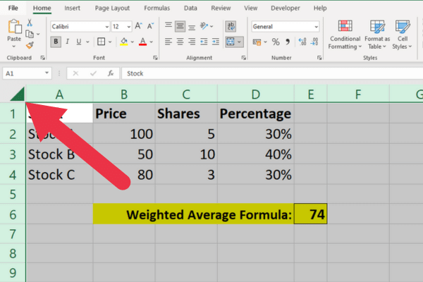
Step 1: Select all cells in the worksheet
You can select all cells by using the keyboard shortcut Ctrl-A.
Alternatively, click the green triangle in the top-left box of the sheet.
Step 2: Open the Format Cells Dialog Box
Right-click on the selected cells and choose “Format Cells” from the drop-down menu.
Alternatively, you can go to the Home tab, click on the “Format” drop-down, and select “Format Cells.”
Step 3: Go to the Protection Tab
In the “Format Cells” dialog box, click on the “Protection” tab. Here, you will see the options for locking and hiding cells.
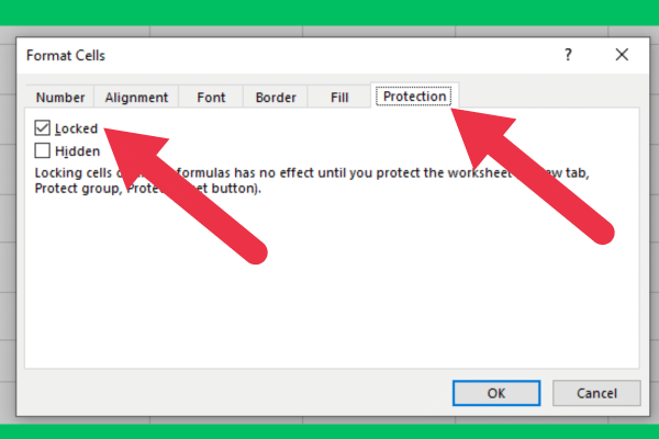
Step 4: Uncheck the Locked Box
To remove locking, uncheck the Locked box. Then, click “OK” to close the dialog box.
Step 5: Select the Cells You Want to Lock
Now, select the cells that you want to lock.
You can select a single cell or multiple cells by holding down the Ctrl key while selecting.
Step 6: Open The Protection Tab In The Format Cells Dialog box
Repeat steps 2 and 3 to go back to the Protection Tab.
Step 7: Check the Locked Box
To lock the selected cells, tick the Locked check box. Then, click “OK” to close the dialog box.
Step 8: Protect the Worksheet
Finally, go to the “Review” tab and click on “Protect Sheet.”
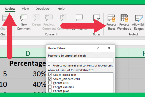
In the “Protect Sheet” dialog box, you can choose the options you want to apply to the protected cells.
You can choose to allow certain users to edit the cells in an Excel worksheet, or you can set a password to prevent unauthorized access.

The default options are often all you need. They will allow users to view and copy data in the locked cells, but they won’t be allowed to edit the cells.
How to Allow Certain Users to Edit Locked Cells
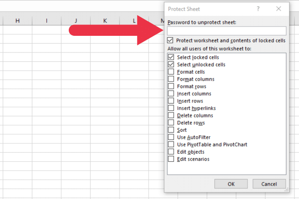
You have learned how to lock cells in Excel to prevent accidental editing. However, users can simply unprotect the worksheet to remove the locking.
You may want to prevent all but a few users from being able to do so. This is achieved by setting a password that users must enter to remove the protected property.
The option is available at the top of the Protect Sheet dialog box.
How to Lock Formulas in an Excel Worksheet
When you use formulas in your worksheet, you may want users to be able to edit the data cells but not change the formula cells.
That’s easy to achieve when you just have a handful of formulas. Follow the steps above to lock formula cells.
The task can be more tedious if you have many formulas in a worksheet. For example, working with frequency and distribution charts may require many formulas on an Excel sheet.
Thankfully, Excel gives us a shortcut. Again, before you protect specific cells, unlock the entire worksheet using the steps in the previous sections.
Now, follow these steps to select all formulas:
Go to the Home tab.
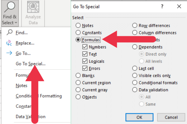
Expand the “Find & Select” drop-down menu in the Editing section (far right).
Choose “Go To Special”.
Tick the Formulas option to select formulas.
Click OK.
Excel has now selected all the cells with formulas. You can use the Format Cells window for locking specific cells.
Spotting unlocked cells with formulas
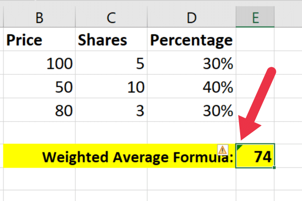
If there is a formula in an unlocked cell, Excel shows a yellow triangle with an exclamation mark as a warning sign. When you click on the triangle, you will see hints as to the problem.
The solution is to restrict users from editing the formula by ensuring that the cell or cells are locked.
This picture shows the warning sign. Although the other cells are not locked, they do not show the symbol.
The problem can be rectified with these steps:
select the cell or specified range.
click format cells.
to protect cells, tick the locked checkbox on the Protection tab.
Click “protect sheet” in the Review tab to protect the sheet.
How to Lock Pivot Tables
It can take time and effort to set up all the data for a pivot table in Excel. When sharing the spreadsheet, you may not want other people to be able to change the underlying data.
Follow the same steps that we detailed to unlock all cells. Then, lock your pivot tables by selecting all the cells that contribute to them. This includes:
Headers.
Data cells.
Any additional rows or columns that contain explanatory or supporting details.
Finally, protect the sheet using the Review tab in the ribbon.
How to Unlock Cells When You Forget Your Password

If you forget the password you set to protect a worksheet, there is no easy way to unlock the cells due to the general need for password protection.
You may need to recreate the worksheet from scratch or from a backup copy if you have one. It is always a good idea to store your passwords securely in case you need them later.
If you want to explore a workaround, it’s possible to write a VBA script that may unprotect the Excel spreadsheet. However, this may be against the terms of use of the software.


