
So you’ve managed to master the basics of Excel – kudos to you! Now, you’ve decided to kick things up a notch and dive into the more advanced stuff, right? Well, you’re in luck because we’ve put together a handy intermediate Excel cheat sheet just for you!
This Microsoft Excel intermediate cheat sheet covers a wide range of topics that will level up your skills in numerical analysis, text processing, and complex date and time logic.
By having the Excel Intermediate Cheat Sheet as a desktop reference, you can dive deep into the more powerful formulas and functions of Microsoft Excel.

Now, make sure to read on, but also print and save the cheat sheet below!
Let’s get started!
Intermediate Math Formulas
Our beginner cheat sheet covered the most common beginner math functions such as the SUM function. Intermediate users should become familiar with these more complex functions:
ABS() returns the absolute value of a number.
SQRT() returns the square root of a number
RAND() provides a random number between 0 and 1
Conditional Logic
Intermediate users should also know how to perform math calculations based on multiple conditions using these functions:
SUMIFS(sum_range, criteria_range1, criteria1, [….])
COUNTIFS(criteria_range1, criteria1, [criteria_range2, criteria2], …)
AVERAGEIFS(criteria_range1, criteria1, [criteria_range2, criteria2], …)
The functions evaluate the criteria provided and produce a logical value of TRUE or FALSE.
Let’s say you have the following sales data in columns A, B, and C:
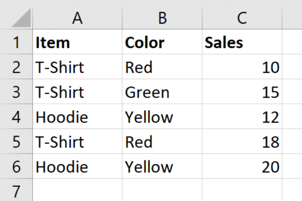
To calculate the sum of sales for red t-shirts, use the SUMIFS formula:

=SUMIFS(C2:C6, A2:A6, “T-Shirt”, B2:B6, “Red”)
To count the number of rows with red t-shirts, use the COUNTIFS formula:
=COUNTIFS(C2:C6, A2:A6, “T-Shirt”, B2:B6, “Red”)
To calculate the average sales for red t-shirts, use the AVERAGEIFS formula:
=AVERAGEIFS(C2:C6, A2:A6, “T-Shirt”, B2:B6, “Red”)
Intermediate Statistical Formulas
Aside from basic functions like MIN and MAX, Excel has a wider range of statistical formulas for intermediate users. Here are some of the most useful:
MINA
MAXA
COUNTA
COUNTIF
1. MINA and MAXA
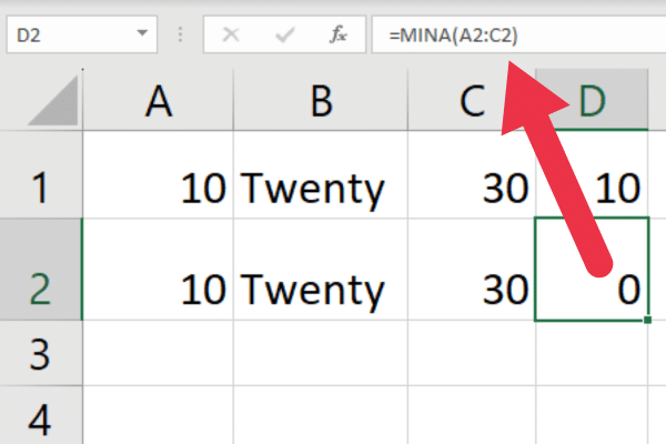
The more commonly used MIN and MAX functions ignore text values.
The alternative MINA and MAXA functions consider both text and numbers when looking for the highest or lowest values. Text values are evaluated as if they were zero.
The differences are shown in the picture below. The first row evaluates a minimum value of 10, while the second row evaluates as 0 due to the presence of a text value.
2. COUNTA and COUNTIF
The COUNTA function is used to count the number of non-empty cells in a range.
The COUNTIF function is less specific in that is used to count the number of cells within a range that meet a specific condition or criteria.
You can also use these functions to count the number of distinct values in a column. This video shows how to do so.
Excel Formulas for Financial Analysis
There are several formulas you will want to use when performing financial analysis such as forecasting investments:
PRODUCT(number1, [number2…])
QUOTIENT(numerator, denominator)
LOG(number, [base])
1. PRODUCT Function
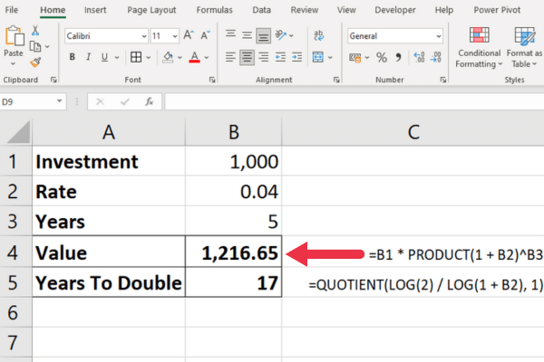
Suppose you want to calculate the future value of an initial investment of $1,000 (cell B1) at an annual interest rate of 4% (cell B2) after five years (cell B3).
Use the PRODUCT function to calculate the future value with this formula:

=B1 * PRODUCT(1 + B2)^B3
This formula will return the future value of your investment.
2. QUOTIENT and LOG Functions
The next step is to calculate how many years it will take for an investment to double in value at the given interest rate.
Use the QUOTIENT function in combination with the LOG function to calculate this as follows:
=QUOTIENT(LOG(2) / LOG(1 + B2), 1)
This formula will return 17 with the sample data, indicating that it will take 17 years for the investment to double in value at an annual interest rate of 4%.
This picture shows the formulas in an Excel worksheet:
Functions for Investment Scenarios
These are some functions that are suitable for specific financial scenarios. One of them may be exactly what you need:
NPV – The NPV (Net Present Value) function will calculate the net present value of an investment based on a series of future cash flows based on a discount rate.
ACCRINT – The ACCRINT function calculates the accrued interest of a security that pays periodic interest. This is useful for determining the interest earned on a security since the last payment date up to a given settlement date.
INTRATE – The INTRATE function calculates the interest rate for a fully invested security.
PMT – The PMT function calculates the total payment on a debt security.
IRR – The IRR function provides the internal rate of a return.
YIELD – The YIELD function provides the yield of a security based on interest rate, face value, and maturity.
Intermediate Excel Date and Time Formulas
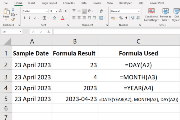
The basic date and time functions in Excel include the NOW and TODAY functions for the current date. Intermediate users should also know how to extract components from a given date using:
DAY(date)
MONTH(date)
YEAR(date)
The formula =MONTH(“23 April 2023″) will return a result of 4 for the 4th month. Similarly, the DAY and YEAR functions will return 23 and 2023 respectively.
1. Intermediate Month Functions
Intermediate users will sometimes deal with adding or subtracting months to a date and finding the end of a month.
EDATE(start_date, number_of_months)
EOMONTH(start_date, number_of_months)
For example, the formula =EDATE(“23 April 2023”, 2) will calculate the date two months later.
The formula =EOMONTH(23 April 2023”, 2) calculates the end of the month two months later.
The result is “30 June 2023”, which takes into account that there are only thirty days in June. If you specify 3 months, the result will be “31 July 2023”.

2. Intermediate Week Functions
You can use a combination of the SUM and WEEKDAY functions to count the number of whole workdays within a range of dates.
The WEEKDAY function returns the day of the week for a given date. The second parameter determines the numbering system with the default being Sunday to Saturday.
If you have a series of dates in a cell range of B1:B40, use this formula to calculate the workdays:
=SUM(–(WEEKDAY(B1:B40,2)>5))
3. Intermediate Time Functions
The YEARFRAC function calculates the fraction of a year between two dates.
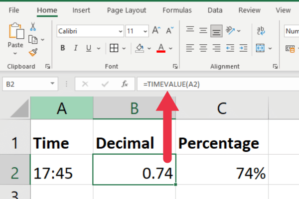
The TIMEVALUE function is used to convert a time represented as text into a decimal number representing the proportion of a 24-hour day.

The result is an Excel serial number where 1 represents a full 24-hour day, 0.5 represents 12 hours, 0.25 represents 6 hours, and so on.
Suppose you have a time in text format “17:45” in cell A1 and you want to convert it into a decimal number. This is the formula:
=TIMEVALUE(A1)
The value 0.74 represents the proportion of the 24-hour day that has passed by at the time of fifteen minutes before six o’clock.
Take to to change the time cell from a time format to a text format. You may want to format this as a percentage to be clearer.
Excel Functions for Conditional and Logical Algebra
Conditional and logical functions are essential for decision-making in Excel. The following functions can be combined with the more basic Excel formulas for powerful logic:
IF(condition, value_if_true, value_if_false):
AND(condition1, condition2, …)
OR(condition1, condition2, …)
NOT(condition1, condition2, …)
The IF function evaluates a condition and returns different values depending on whether the condition is true or false.
The AND, OR, and NOT functions check which conditions are true and let you make decisions accordingly.
Here are some examples based on the sales data we used before.
1. IF Function
Suppose you want to display the text “Low Sales” if the sales for the items are less than 15. If the sales are higher, you want to display “High Sales” in a new column.
Use this formula and copy it down to the other rows:
=IF(C2<15, “Low Sales”, “High Sales”)
2. AND Function
Suppose you want to display TRUE or FALSE for t-shirts with at least 15 sales. Use this formula:
=AND(A3=”T-Shirt”, C3>=15)
3. OR Function
Suppose you want to test multiple conditions and return TRUE if any of the conditions are met and FALSE otherwise, then you’d use the OR function.
For instance, if we have scores of a test in cells A1 and B1, and we want to know if either score is above 80, we could use: =OR(A1>80, B1>80). This will return TRUE if either score (or both) is over 80, and FALSE if both are 80 or less.
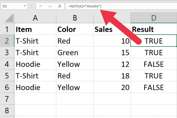
4. NOT Function
Suppose you want to check if the item is not a hoodie. Use this formula:
=NOT(A2=”Hoodie”)
Referencing Cells
A beginner will quickly become familiar with using absolute and relative references such as $A$1 or B2. Intermediate users should become familiar with using indirect references, indexes, and offsets:
INDIRECT(ref_text)
INDEX(range, row_num, column_num)
OFFSET(reference_cell, rows, columns):
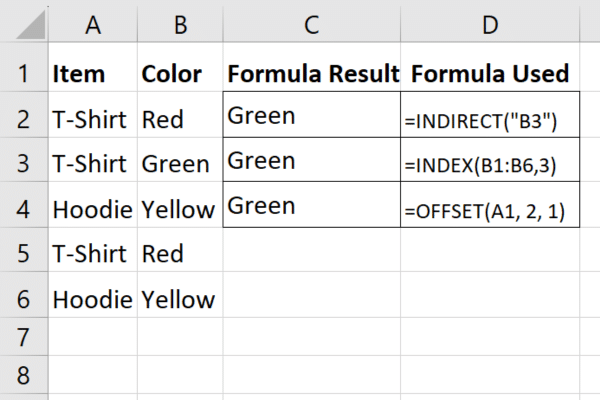
1. INDIRECT Function
The INDIRECT function returns the value of the specified cell reference entered as text. To reference cell B3, use this formula:
=INDIRECT(“B3”)
The advantage over using simple cell references is that this function gives you a dynamic reference. This means that Excel automatically updates the reference when the structure of the spreadsheet changes e.g. a row is deleted.
2. INDEX Function
The INDEX function is used to reference cells within a specified range based on row and column numbers.
To reference cell B3 in a table of six rows, use this formula:
=INDEX(B1:B6, 3)
3. OFFSET Function
The OFFSET function returns a cell or range that is a specified number of rows and columns away from a reference cell.
If you want to display the cell value that is two cells across and one cell down from A1, use this formula:
=OFFSET(A1, 2, 1)
Here are the formulas in action:
Intermediate Text Formulas
Beginners should know text functions like LEFT, which extracts one or more characters from the left side of a string. A power user should be familiar with functions like these:
TEXTJOIN(delimiter, ignore_empty, text1, [text2, …])
REPLACE(old_text, start_num, num_chars, new_text)
SUBSTITUTE(text, old_text, new_text, [instance_num])
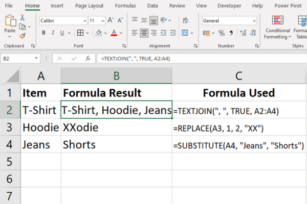
1. TEXTJOIN Function
The TEXTJOIN function concatenates cells with the delimiter that you provide. You can also specify where to ignore blank cells.
To produce a comma-delimited list of some items in column A, use this formula:
=TEXTJOIN(“, “, TRUE, A2:A4)
2. REPLACE Function
The replace function lets you specify the starting position and length of the string you want to swap into the target.
To replace the first two characters of a string with “XX”, use this formula:
=TEXTJOIN(A2, 1, 2, “XX”)
3. SUBSTITUTE Function
The substitute function replaces specified occurrences of a text string within another text string with a new text string.
To replace occurrences of the word “Jeans” with “Leggings”, use this formula:
=SUBSTITUTE(A3, “Jeans”, “Leggings”)
Here are the formulas in action:
Intermediate Lookup Formulas
Common lookup functions like VLOOKUP and MATCH are covered in the beginner’s cheat sheet.
Intermediate users should get familiar with the CHOOSE lookup function:
CHOOSE(index_num, value1, [value2, …])
The CHOOSE function returns a value from a list of values based on a specified index number.
Suppose you have a column of t-shirt sizes labelled as 1, 2, or 3. You want to display a category of small, medium, and large respectively in the same row. Use this formula:
=CHOOSE(A1, “Small”, “Medium”, “Large”)
Formulas for Handling Microsoft Excel Errors
The beginner cheatsheet listed the typical error messages you will see when working with Excel. Intermediate users should be able to use formulas to handle the errors gracefully.
IFERROR(value, if_error)
IFNA(value, value_if_na)
1. IFERROR Function
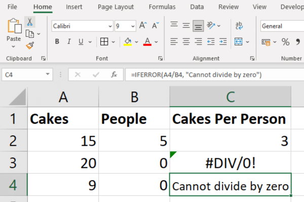
Division by zero errors are common but Excel’s default display of #DIV/0! won’t be clear to every user.
Use the IFERROR function to replace the standard error with “Cannot divide by zero” with this formula:
=IFERROR(A1/B1, “Cannot divide by zero”)
This picture shows the raw error in the third row and the IFERROR function handling the fourth row.
2. IFNA Function
The IFNA function in Excel is used to catch and handle #N/A errors.
Another section of this cheat sheet showed the CHOOSE function. This function will return a N/A error if the index number is not an integer.
Suppose a t-shirt size has been entered as 1.5, with the user mistakenly thinking that this will show a category somewhere between small and medium. Instead, it will show a #N/A error.
To provide a more helpful error, use this formula:
=IFNA(CHOOSE(A2, “Low”, “Medium”, “High”), “Invalid index”)
Formula and Function Shortcuts
There are several keyboard shortcuts that can make you work more efficiently with your worksheet.
F2: Edit the active cell and position the insertion point at the end of the cell contents.
F9: Calculate and display the result of the selected portion of a formula.
Ctrl + Shift + Enter: Enter an array formula.
Shift + F3: Open the Insert Function dialog box.
Esc: Cancel the entry of a formula and revert to the original cell contents.
Some of these Excel shortcuts might not be available in all languages or keyboard layouts.
Intermediate Cell Formatting
In financial analysis, proper formatting for cells containing numbers, dates, and currencies is crucial. To format cells, follow these steps:
Select the cells you want to format.
Right-click on the selected cells and choose “Format Cells.”
Select the appropriate category (e.g., Number, Currency, Date) and apply the desired format.
Some common formatting types to consider in finance include:
Currency: $1,234.56
Percentage: 12.34%
Accounting: ($1,234.00)
Date: 10-May-2023
Final Thoughts
As you become more comfortable with the various formulas and functions highlighted in this cheat sheet, you’ll find yourself better equipped to handle increasingly complex tasks and projects.
Practice is key to mastering any skill, so don’t be afraid to experiment with these formulas in your day-to-day work. They will bring your expertise from beginner level to intermediate level.
This is just a taste of what Excel’s intermediate functions can do to simplify your work, streamline your analyses, and help you uncover insights from your data.
The real magic happens when you start combining the functions in our cheat sheet and tailor them to suit your unique needs. So, don’t stop here. Keep exploring, keep experimenting, and you’ll find that Excel is not just a tool, it’s a game-changer!
Feel like you want to take things to the next level? Check our Excel Advanced Formulas Cheat Sheet.


