
Power Query is a powerful business intelligence tool in Excel that enables you to import, clean, and transform data according to your needs. If you have ever spent hours cleaning up data (we have) or struggled to merge data from various sources (we also have), this feature will make your life easier.
The best way to learn how to use Power Query in Excel is to perform some common tasks like importing data and using the Power Query Editor to transform the resulting tables and combine the data.
This article gets you started by showing clear Power Query examples with step-by-step guides. By mastering Power Query, you can elevate your work to the next level.

Are you ready? Let’s do this.
How to Know if You Can Access Power Query
Before you start using Power Query, you need to be sure that you have a version of Excel that has the feature.
Here’s a brief overview of Power Query by version:
Excel 2010 and Excel 2013: available as an add-in that needs to be downloaded and installed.
Excel 2016: integrated into Excel as “Get & Transform”.
Excel 2019: improved performance and functionality.
Excel 2021 and Excel for Microsoft 365: integration with cloud data sources.
Excel for Mac: only available from Microsoft 365 version 16.69 and later.
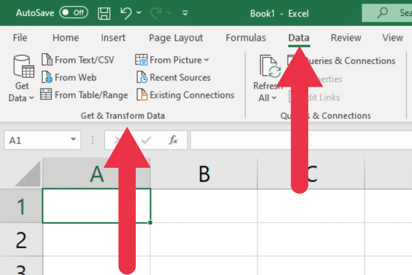
To verify that the tool is integrated in your Excel workbook (2016 or later), go to the Data tab and look for the “Get & Transform Data” section in this picture:
If you have Excel 2010 or 2013 on Windows, you can download, install and enable the Power Query add-in.
How to Import Data With Power Query
The Power Query tool allows you to import and connect to a wide range of data sources:

Files, including CSV, XML, and JSON formats
Web URLs or API endpoints
Databases, including Access, SQL Server, Oracle, and most modern databases
Azure services, SharePoint files, and OData feeds
The easiest data source to start with is a simple CSV file with several lines of data. Create a text file and add these four first and last names, separated by a comma:
Joe, Bloggs
Anne, Ryan
James, Stewart
Mary, Brown
Be sure to save the file with the .CSV extension. Your file will look like this:

To load the data with Power Query, follow these steps:
Go to the Data tab.
Click the “Get Files” button in the Get & Transform Data tab.
Select your sample file.
You may have to wait a few seconds for the tool to pull in the data to the preview pane. Power Query uses quite a lot of machine resources even for a small import, so please be patient people.
Tip: shut down other applications to speed up performance.
Power Query will display the “Text/CSV Import” window with a preview of your data.
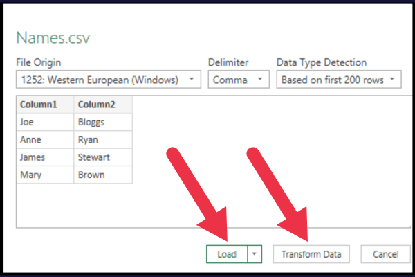
If the data looks correct, you can proceed to load or transform the data:
the Load button will load data directly into Excel.
the Transform Data button lets you modify the data before loading it.
Did you notice that the sample file didn’t have a header? If it’s loaded straight into Excel, the headers will be “Column 1” and “Column 2”.
Instead, you can pull the data into the Power Query editor and make some changes. To do so, click the “Transform Data” button.
The Power Query Editor now opens, which brings us to the next section.
How to Use The Power Query Editor
In this section, we’ll explore some essential aspects of working with the Power Query Editor.
Data Preview
In the Data Preview area, you can view and interact with your imported data. You can filter rows, modify column data types, and reshape the data to suit your needs.
When you’re finished, Excel will load the transformed data into a worksheet.
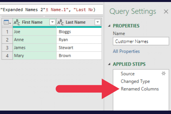
Using the sample file, you can edit the column names directly in this pane.
To do so:

Right-click the column header.
Click “Rename” in the drop-down menu.
Type the preferred names into the header boxes.
As you make changes, the “Applied Steps” section on the right of the preview pane updates to reflect each transformation, allowing you to track and modify your data processing steps as needed.
Properties
Setting properties for your queries is essential for organizing and tracking your work.
The Query Settings pane is on the right of the Power Query window.
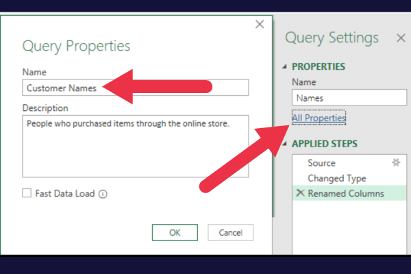
Click the “All Properties” link.
Edit the name of the Query to be descriptive.
Add a description to provide more information.
It’s easy to forget what last week’s queries were set up to do. In this case, the query name has been changed and a description has been added that gives the purpose of the query.
If you want to learn more about the options available, check out this overview of the Power Query Editor.
How to Work With Multiple Data Sources
The Power Query Editor offers two primary methods for combining data from multiple sources: appending and merging.
Appending joins tables vertically, stacking them on top of each other. Merging allows you to join tables based on common columns.
To see how this works, create a second small CSV file with the same structure as the first. This time, put two names (first and last) into the file:
Joe, Bloggs
Laura, Cane
Notice that one of these names is repeated from the previous file.
Now follow these steps to pull the data into your Microsoft Excel workbook.
Close the Power Query Editor window and save your changes.
Add a new worksheet.
Follow the steps in the previous section to import the second file.
Click the Transform button.
Rename the column headers as “First Name” and “Last Name”.
The right pane in the Excel worksheet shows the current Queries & Connections. You should now see two queries in the pane.

How to Append Data With Power Query
In this section, you will append the second sample CSV file to the first.
Follow these steps to append data:
Right-click on the first table (Customer Names) in the Queries & Connections pane.
Choose “Edit” to open the table in the Power Query Editor.
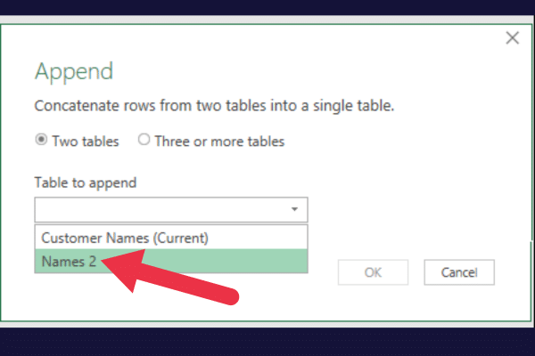
Click on Append Queries in the Combine section.
Choose the second table from the drop-down list of tables to append.
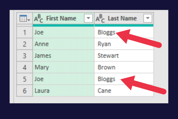
The result will be two extra rows in the first table.
Notice that one row is repeated – this is how the append operation works. It adds the data from one table into another, regardless of whether the data already exists.
You can remove the duplicate data in the Power Query Editor with these steps:
Click on the “First Name” column header.
Hold the “Ctrl” key (or “Cmd” key on Mac).
Click on both column headers.
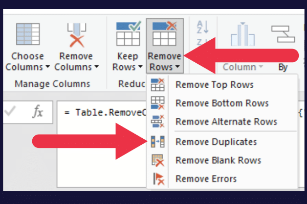
Click on “Remove Rows” in the Home tab of the Power Query Editor ribbon.
Select “Remove Duplicates” from the drop-down menu.
How to Merge Data With Power Query
When you merge data, you must choose the matching columns between the queries.
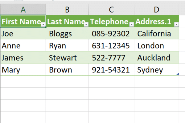
Suppose you have two comma-delimited files where one contains customer phone numbers and the other contains addresses. The two files look like this:

Follow the instructions in the previous sections to load each file into its own power query. Then you can practice merging the tables.
In the case of our sample data, both columns (First Name and Last Name) should be picked as the matching columns. Hold down the Ctrl key to pick multiple columns.

Follow these steps:
Right-click on the first table in the Queries & Connections pane.
Choose “Edit” to open the table in the Power Query Editor.
Select “Merge Queries” from the “Combine” group.
Choose the second table in the dropdown list of tables.
Click on the first column in the first table.
Hold down the Ctrl key and click on the second column in the first table.
Hold down the Ctrl key and click on both columns in the second table.
Keep the default join operator as “Left Outer”.
Click “OK” to apply the changes.
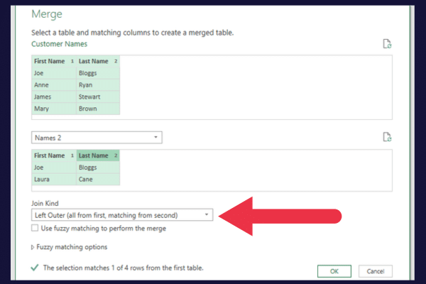
The “Left Outer” join operator ensures that duplicate data is eliminated.
In the Power Query Editor, you’ll see a new column named “Table” or “Nested Table” containing the merged data from the second query.
Click on the expand icon (two arrows) in the header of this column.
Uncheck the “use original column as prefix” box (this avoids long column names).
Click “OK”.
Click “Close and Load”.
The merged table had four columns, with the telephone and address details merged. You may still have a bit of tidying up to do.
For example, you may want to edit the name of the table (Merge1) and the address column in the picture below.
5 Ways to Transform Data With Power Query
Transforming data in your Excel file is made easy with Power Query, allowing you to clean, organize, and manipulate your data effectively.
Some of the most common ways to transform data are:
Expanding and condensing data
Sorting data
Formatting data
Adding and removing columns
Changing data types
1. Expanding and Condensing Data
Expanding and condensing data is important for making your datasets more manageable. Power Query allows you to expand or collapse tables for a more organized view.
The previous section shows you how to expand by including data from related tables.
You can also condense it to only include summarized data based on an aggregation of your choice such as sum, count, or percentage.
2. Sorting Data
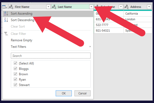
To sort data, you can quickly change the order by ascending or descending values.
Click on the down arrow beside a column name and choose “Sort Ascending” or “Sort Descending”.
3. Formatting Data
The Transform tab in the Power Query Editor provides a lot of options.
For example, the Format drop-down menu lets you change all data in a column or the entire table to upper case or lower case.
4. Adding And Removing Columns
Power Query simplifies the process of adding, deleting, and modifying columns.
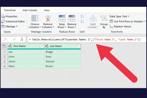
To remove a column, simply right-click on the header of the undesired column and select “Remove.” This will permanently delete the column and all of its data from the table.
To add a new column, select the existing column where you’d like the new one to appear. Then use the “Add Column From Examples” feature to create a custom column or to perform calculations between two or more columns.
5. Changing Data Types
Working with consistent and accurate data types is crucial for accurate analysis. Power Query allows you to change data types easily:
Right-click on the column header.
Choose “Change Type”.
Select the desired data type from the list provided.
Changing data types can be particularly useful when dealing with percentage data.
For example, you may need to convert decimal points to percentages or convert text-based percentages to numeric ones for easier calculation and comparison.
Working with Formulas and M Language
When using Power Query in Excel, you’ll encounter the M Language, which is the heart of creating advanced formulas, manipulating data, and producing powerful queries. In this section, you’ll learn about:
the Formula Bar
M code
the essential elements of M Language syntax
Formula Bar
The Formula Bar in Excel’s Power Query editor is the area where you’ll input your formulas and M code.
To use it, go to the Power Query editor by selecting a query from the Queries & Connections pane. The Formula Bar is located above the data preview pane.
Writing And Modifying M Code
To create versatile and powerful queries in Excel, you’ll need to write and modify the Power Query language known as M code. Here are some tips on how to get started:
Use the Applied Steps pane to write step-by-step code, making it easy to track and modify your query’s logic.
Combine M code with an Excel table, pivot tables, and external data sources, like Azure and text files, to create dynamic and automated reports.
Adjust the Query Options to refine your data loading preference and improve performance.
As you familiarize yourself with M code, you’ll find you can automate and optimize many processes, making your data analysis in Excel more efficient and powerful.
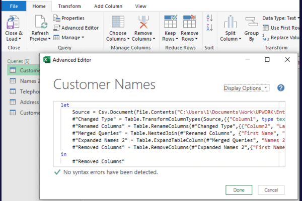
To view the code behind a query, follow these steps:
Open the query in the Power Query Editor.
Click on “Advanced Editor” in the Home tab.
This is the code behind our sample merged table (yours may look different):
What is M Language Syntax?
Understanding M Language syntax is crucial for creating effective Power Query formulas. Keep the following points in mind:
M Language is case-sensitive, so be careful with capitalization.
Use square brackets [] for referencing columns, records, and lists.
To reference a previous step in your query, use its variable name (e.g., #”Step Name”).
Output a query formula step with the “in” statement.
As you gain experience with Power Query language flow, you’ll discover new ways to transform and analyze your data, making your Excel workbooks an even more valuable asset.
Check out the video below, it’s time to get out the scrubbing brush and clean up your messy data.
How to Refresh Data Connections
One of the key features of Power Query is the ability to refresh your a Power Query connection easily.
When your data sources have been updated, and you need the latest information in your workbook, you can refresh the data connections in the Queries & Connections pane.
If you don’t see the pane on the right of your worksheet, you can open it by going to the Data table and clicking on “Queries & Connections”.
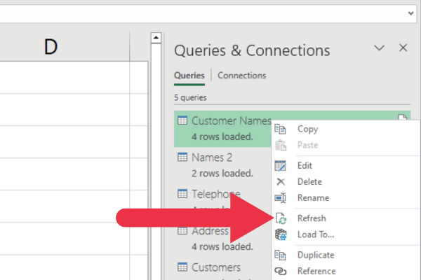
When the Queries & Connections pane is open, it lists all the queries. Follow these steps:
Right-click on the query you want to refresh.
Select Refresh from the context menu.
This will update your workbook with the latest data from your connected data sources.
How to Integrate Power Query With The Data Model
Excel’s data model is a powerful feature that allows you to create business intelligence tools, like pivot tables, based on data relationships.
The data model is basically a hidden database that holds the imported data and relationships between tables.
It is part of the Power Pivot feature which is in-built into current versions of Excel. You may have to install Power Pivot as an add-in to access it in previous versions).
You can integrate your Power Query data connections with the data model with these steps:
Load your data using Power Query as described in previous sections.
Instead of loading it directly into the workbook, choose Load To from the Load menu.
Select Add this data to the Data Model checkbox in the Import Data dialog box.

How to Automate With Power Query And VBA
With VBA (Visual Basic for Applications) integration, you can create custom data connections and automate data transformation steps in Power Query.
You can leverage your existing VBA skills to build advanced data models by incorporating data from platforms like Microsoft Access, SharePoint, and Analysis Services.
Although Power Query does not have native support for VBA, you can use VBA code to open, refresh, and manipulate Power Query queries indirectly.
This allows you to create powerful, automated data workflows and streamline your data analysis process.
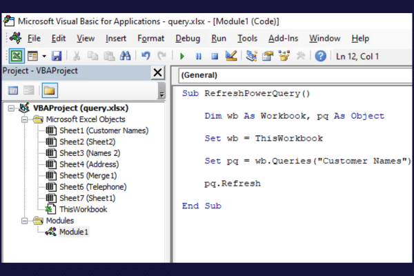
Here is some sample code that refreshes a power query in the current workbook.
:
Dim wb As Workbook, pq As Object
Set wb = ThisWorkbook
Set pq = wb.Queries(“Customer Names”)
pq.Refresh
Here is the code within an Excel VBA macro:
Power Query Advanced Features
Excel’s Power Query offers a plethora of advanced features to simplify and enhance your data analysis process. By learning how to effectively use these features, you can take your data analysis skills to a whole new level.
The built-in data analysis tools include:
Conditional columns for applying complex logic to your data transformations.
Grouping and aggregation functions to summarize your data in a meaningful way.
Pivot and Unpivot operations to reshape your data for easier analysis.
You’ll find many of these features in the Transform tab in the Power Query Editor.
Additionally, you can connect Power Query to Business Intelligence tools like Power BI for more advanced data analysis and visualization options.
Collaboration and Sharing
Sharing your data connections, queries, and transformations with your team members is essential for effective collaboration.
You can share a workbook with queries by saving it to a network drive, SharePoint, or some other shared storage location.
You can also export the M code behind a single query with these steps:
Edit the query in the Power Query Editor.
Click on “Advanced Editor” in the Home tab.
Copy the entire M code in the Advanced Editor window.
Open a text editor (e.g., Notepad) and paste the copied M code into the text editor.
Save the text file and send it to your colleague.

Let’s Wrap This Up
With an array of features and its user-friendly interface, Power Query is an essential tool for Excel users looking to work effectively with external data.
This valuable feature helps streamline the process of creating reports, data cleansing, and performing complex analyses on your data tables. Using
Power Query ultimately saves you time and increases efficiency when working with Excel files.


