
Are your cells overloaded with messy data and you just want to extract a piece of data from each cell? That’s where substrings come into play.
Substrings are like magic scissors for your data. If you ever wanted to know how to pull out specific parts of text or numbers from your Excel cells, stick around.
Here are some handy methods with Excel text functions for extracting substrings:

- To extract a substring from the left side – Use the LEFT function
- To extract a substring from the right side – Use the RIGHT function
- To extract a substring from the middle – Use the MID function
- To extract a substring before a specific character – Use the TEXTBEFORE function
- To extract a substring after a specific character – Use the TEXTAFTER function
In this article, we’re going to break down everything you need to know about Excel substrings, step by step!

We’ll make it easy, promise!
What Are Substrings in Excel?
A substring in the context of Excel refers to a smaller portion or segment of a text string that exists within a larger text string.
Let’s assume that you have a text entry “12-AB” in a cell of your Excel file.
A substring refers to any part of the “12-AB”. So, substrings could be;
- 12
- AB
- 1
- 2
- A
- B
- 12-A
- 2-A
Similarly, any section of an original text string can be considered a substring. You have the flexibility to extract substrings from the beginning (left), middle, or end (right) of a text string.

While there is no direct Excel SUBSTRING function available, Excel enables users to extract these substrates using various text functions, such as LEFT, MID, RIGHT, TEXTBEFORE, and TEXTAFTER text functions.
Excel also offers other text functions like FIND, LEN, SUBSTITUTE, TRIM, and REPT. These can be used in combination with the main substring functions to gain more control over the resulting substring structure and content.
Employing substrings with correct syntax and accurate knowledge, users can handle extensive text manipulation tasks in Excel with confidence and ease.
Now that we’ve gone over the fundamentals, let’s go over how you can extract a substring in Excel in the next section!
How to Extract Substrings in Excel – 5 Methods
In this section, we’ll explore the basic Excel functions used to extract substrings. These include the LEFT, RIGHT, MID, TEXTBEFORE, and TEXTAFTER functions.
1. LEFT Function
When you want to extract a substring from the beginning of a text string, you can easily use the Excel LEFT function.
The LEFT function allows you to extract a specified number of characters from the left side of a cell. The LEFT function syntax is as follows:
LEFT(text, [num_chars])
- text: The cell or text value from which to extract the characters
- num_chars (optional): The number of characters to extract from the left side of the text
Example:
Column A of the below table has some product codes. The first two characters represent the size of the product.
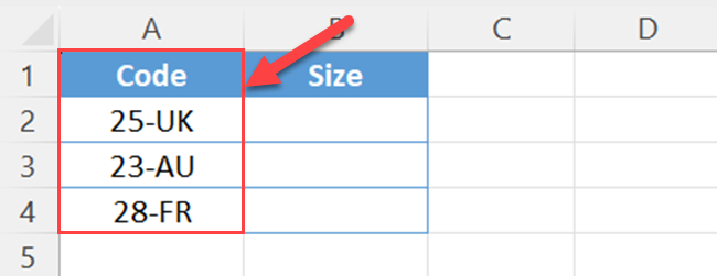
Now, assume that you want to extract the size of each product in Column B.
Then, you can use the Excel LEFT function to extract the first two characters.
=LEFT(A2,2)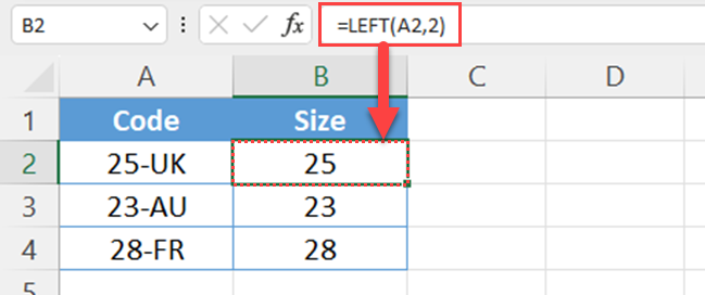
In the above function, the text is A2. As the size of the product represents the first two characters of the product code, the number of characters to be extracted is 2.
2. RIGHT Function
Occasionally, you might need to grab a part of text from the tail end of a text string. When this happens, you can use the Excel RIGHT function.
The RIGHT function extracts a specified number of characters from the right side of a cell. The RIGHT function syntax is:
RIGHT(text, [num_chars])
- text: The cell or text value from which to extract the characters
- num_chars (optional): The number of characters to extract from the right side of the text
Example:

Column A of the below table has some product codes. The last two characters represent the country code of the product.
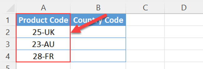
Now, assume that you want to extract the country code of each product to Column B.
Then, you can use the Excel RIGHT function to extract the last two characters.
=RIGHT(A2,2)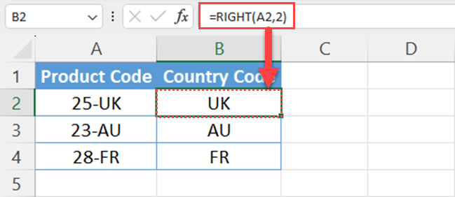
In the above function, the text is A2 as we want to extract the substring from the cell reference A2. As the country code of the product represents the last two characters of the product code, the number of characters to be extracted is 2.
3. MID Function
Sometimes, there’s a need to get a part of a text string right from the middle. For these situations, you can make use of the Excel MID function.
The MID function allows you to extract a substring from a cell, starting at a specified position and for a specified number of characters. The MID function syntax is:
MID(text, start_num, num_chars)
- text: The cell or text value from which to extract the substring
- start_num: The starting position of the substring extraction
- num_chars: The number of characters to extract
Example:
Column A of the below table details product codes. The character that is between two hyphens represents the color code of the product.
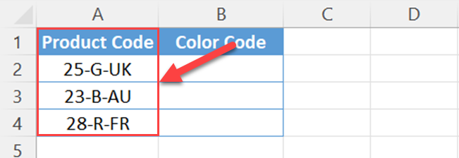
Now, assume that you want to extract the color code of each product to Column B.
Then, you can use the Excel MID function to extract the color code character.
=MID(A2,4,1)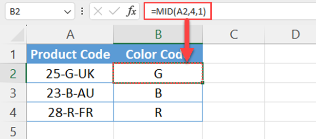
In the above function, the text is A2 as you want to extract the substring from the cell A2. Then, you have to enter, the starting position of the color code. In this case, it is 4.
Finally, you have to enter how many characters you want to extract from the selected text string. In this example, the Color Code column is represented using 1 character. So, 1 is entered for the last argument.
4. TEXTBEFORE Function
At times, you need to pull out some text that comes before a particular character. In Excel, there’s a new text function called TEXTBEFORE that can help you do just that.
The TEXTBEFORE function helps you to extract characters before a given character. The TEXTBEFORE function syntax is as follows:
TEXTBEFORE(text,delimiter,[instance_num],[match_mode],[match_end],[if_not_found])
- text: The cell or text value from which to extract the characters
- delimiter: The text that indicates the spot where you want to start extracting the substring.
- instance_num (optional): The occurrence of the delimiter from which you wish to extract the text.
- match_mode: Decides if the text search pays attention to uppercase and lowercase letters.
- match_end: Considers the end of the text as a delimiter.
- if_not_found: The value given back when there’s no match discovered.
Example:
Column A of the below table has some product codes. The country of origin is mentioned before the hyphen in each product code.
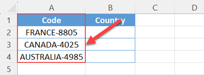
Now, assume that you want to extract the country of origin of each product in Column B.
Then, you can use the Excel TEXTBEFORE function to extract the country of origin from the original text string.
=TEXTBEFORE(A2,"-")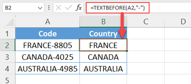
In the above function, the text is A2. The delimiter is the hyphen (-). You have to enter the delimiter within quotes. In this case, you can ignore all other optional arguments of the function syntax.
5. TEXTAFTER Function
Sometimes, you may need to grab a part of the text that comes after a specific character. Good news: Excel has a brand-new text function called TEXTAFTER to help you do just that!

The TEXTAFTER function helps you to extract characters after a given character. The TEXTAFTER function syntax is as follows:
TEXTAFTER(text,delimiter,[instance_num],[match_mode],[match_end],[if_not_found])
- text: The cell or text value from which to extract the characters
- delimiter: the text that marks the point after which you want to extract the substring
- instance_num (optional): The instance of the delimiter after which you want to extract the text
- match_mode: Determines whether the text search is case-sensitive
- match_end: Treats the end of the text as a delimiter
- if_not_found: Value returned if no match is found
Example:
Column A of the below table has some product codes. The country of origin is mentioned after the hyphen in each product code.
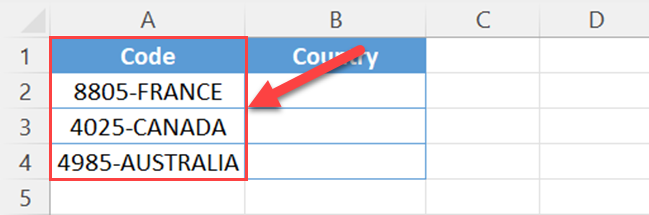
Now, assume that you want to extract the country of origin of each product in Column B.
Then, you can use the Excel TEXTAFTER function to extract the country of origin from the original text string.
=TEXTAFTER(A2,"-")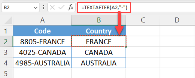
In the above function, the text is A2. The delimiter is the hyphen (-). You have to enter the delimiter within quotes. In this case, you don’t need to use all the arguments of the function. You can use only the two required arguments.
It’s important to note that the TEXTBEFORE and TEXTAFTER functions are currently available only for Microsoft 365 users and Excel web users.
If you’re not a Microsoft 365 user or an Excel web user, you have to use some advanced Excel functions to extract the substring in the last two examples.
The Flash Fill Function
Another handy tool in Excel is the Flash Fill function. This feature automatically recognizes patterns in your data and fills in the rest of the cells by simply typing the desired output in one cell.
Although it’s not a specific substring function, Flash Fill can be used to manipulate text and extract substrates without using any formulas.
To use Flash Fill:
- Type the desired output in the cell next to your input data.
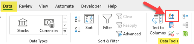
- Press CTRL + E or click the Flash Fill option under the Data tab in the Ribbon.
Example:
Column A of the below table has some product codes. The country of origin is mentioned after the hyphen in each product code.
Now, assume that you want to extract the country of origin of each product in Column B.
Go to cell B2 and type the country of origin of the first product code.

Press Ctrl + E to apply the Flash Fill. If you don’t like Excel shortcuts, go to the Data tab and click the Flash Fill icon in the Data Tools group.
As soon as you apply Flash Fill, you’ll get the country of origin from product codes to column B.
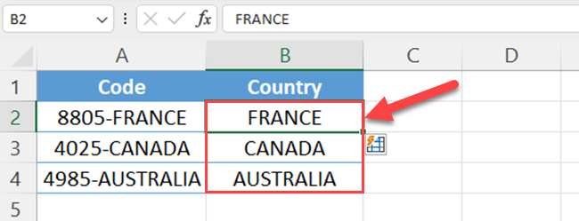
The Excel Flash Fill method is error-prone. So, always remember to check the results when you use this method.
Advanced Excel Functions for Substrings
In this section, we’ll discuss three advanced Excel functions you can use to manipulate substrings, specifically covering the FIND, LEN, and SEARCH functions.
These functions can be very useful in extracting specific parts of text strings and working with text data in your spreadsheets.
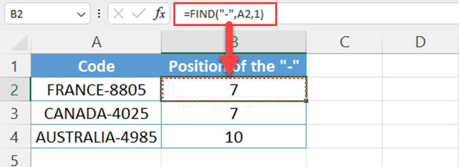
1. FIND Function
The FIND function locates a substring within a text string and returns the position of the first character of this substring. The syntax for the FIND function is:
FIND(find_text, within_text, [start_num])
- find_text: The substring you want to find.
- within_text: The text in which you want to search for the substring.
- [start_num] (optional): The position in the text where the search should begin.
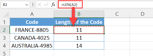
2. LEN Function
The LEN function is used to determine the number of characters in a text string. This function has the following syntax:
LEN(text)
- text: The text string for which you want to count characters.
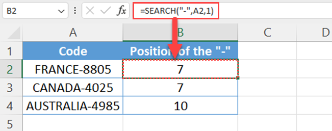
3. SEARCH Function
The SEARCH and FIND functions help to find the position of a given character.
Notably, there are a few key differences, the SEARCH function is not case-sensitive and accepts wildcard characters (* and ?). The syntax for the SEARCH function is:
SEARCH(find_text, within_text, [start_num])
- find_text: The substring you want to find.
- within_text: The text in which you want to search for the substring.
- [start_num] (optional): The position in the text where the search should begin.
Apart from the three functions mentioned earlier, you can also use Excel’s TRIM function and SUBSTITUTE function to dynamically extract a part of the text.
Now, let’s explore how to put these functions to work for substring extraction.
Example:
Column A of the below table has some product codes. The country of origin is mentioned before the hyphen in each product code.
Now, you need to extract the country of origin of each product to Column B. Assume that you’re using an older Excel version, not Microsoft 365.
Then, you can use the below Excel formula to extract the country of origin from the original text string.
=LEFT(A2,FIND("-",A2,1)-1)
You can make formulas just like the above formula to get a specific part of the text string.
Final Thoughts
Understanding substring in Excel is crucial when you need to pick out specific details from a big set of data. It allows you to extract personalized usernames, pull out domain names from email IDs, and more.
Now you’ve learned Excel LEFT, RIGHT, MID, TEXTAFTER, and TEXTBEFORE functions, practice these tools and even combine them for tricky jobs.
In short, this article gives you the basics to be really good at extracting specific text from Excel cells.
If you would like to learn how to extract values before a specific text in Power BI, watch the below video:
Frequently Asked Questions
How do I extract text from a string in Excel?
To extract text from a string in Excel, you can use various functions such as LEFT, RIGHT, MID, TEXTBEFORE, and TEXTAFTER. These functions help you obtain specific parts of a text string based on their position or specific characters.
Which Excel function is used to find specific characters?
The FIND function in Excel helps you locate specific characters within a text string. It returns the position of the character you’re searching for, which you can then use in conjunction with other functions like LEFT, RIGHT, or MID to extract substrings.
How can I get a substring from a cell using an offset?
To obtain a substring from a cell using an offset, you can use the MID function. This function requires three arguments: the text string, the starting position of the substring, and the number of characters to extract.
For example, =MID(A1, 3, 5) would return a substring of 5 characters starting from the 3rd character in cell A1.
What function should be used to find a text from the left or right of a string?
To find a text from the left or right of a string, you can use the LEFT or RIGHT functions, respectively. LEFT extracts a specified number of characters from the beginning of a string, whereas RIGHT retrieves characters from the end of a string.
For instance, =LEFT(A1, 3) will extract the first three characters, and =RIGHT(A1, 2) the last two characters.
How to extract text between two characters in Excel?
To extract text between two characters in Excel, you can use a combination of TEXTBEFORE and TEXTAFTER functions.
For example, =TEXTBEFORE(TEXTAFTER(A2,”-“),”-“).
How can I use the MID function to obtain specific parts of a string?
The MID function can be used to obtain specific parts of a string by specifying the starting position and length of the substring you want to extract.
It requires three arguments: the text string, the starting position, and the number of characters to extract.
For example, =MID(A1, 4, 3) would return a substring of 3 characters beginning at the 4th character in cell A1.


