
At some point, when working in Excel, you will need to find the number of days between two dates.
Fortunately, Excel offers several ways of subtracting dates to get the difference in days between them.
There are three simple ways how to subtract dates in Excel, they are:

- Simple subtraction
- Using the DAYS() function
- Using the NETWORKDAYS() function
There is one older way, the DATEDIF() function, that Microsoft no longer supports. However, the listed three methods are reliable and accurate. You will quickly find the differences between dates for tasks such as project timelines or business analyses.
By the end of this article, you’ll be able to apply each method in your own work to subtract dates to obtain the count of days with ease.
Let’s get into it.
Understanding Dates in Excel
Dates in Excel can sometimes be confusing, as they act as both numbers and text. It makes more sense when you understand that Excel stores dates as serial numbers.
Excel’s date system starts counting from January 1, 1900, which is assigned the serial number 1. Each day that follows is assigned the next number.
For example, January 2, 1900, has a serial number of 2.

You can probably see that this makes it simpler to subtract two dates and find the days between them. Let’s run through the recommended ways to do so.
I suggest you launch a new workbook. Each example I give is a quick tutorial.
My worksheet uses cell B2 and cell C2 for the sample dates. You can use the examples as templates for your work.
1. Using Simple Subtraction To Get The Number Of Days
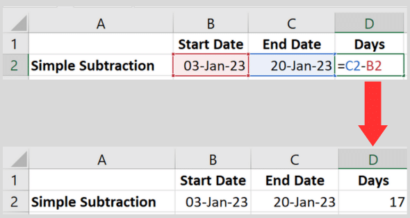
The first method to find the count of days between two dates in Excel is by using simple subtraction (the minus sign). This is the format:
=End-Start
Follow these steps:
- Enter the two dates in separate cells.
- In a new cell, write a formula like this:
=C2-B2 - Press enter.
The resulting value will be the number of whole days between the two dates.
In our example, I entered “3 March 2023” into B2 and “20 March 2023” in cell C2. The result of the calculation was 17.
Cell A2 in the illustration below is simply a description of the method used.
Adding a custom label
If you want to display your result with a custom label, use the following formula:
=C2-B2 & " days"
This formula concatenates the calculated date difference of the cell references with the text ” days”. This provides a more descriptive result.
For example, if there are 17 days between the two dates, the result will be displayed as “17 days”.
2. Using The DAYS Function To Calculate Number Of Days
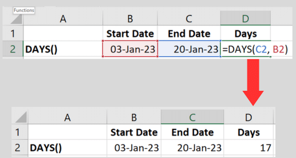
The DAYS Excel function is an inbuilt date function that calculates the days between dates. This is the format:
=DAYS(End, Start)
Follow these steps:

- Enter the two dates in separate cells.
- In a new cell, write a formula like this:
=DAYS(C2, B2) - Press enter.
The resulting value will be the count of whole days between the two dates.
I used the same dates from the previous example to test the function. The resulting number was the same.
The result will always be a whole number. If you prefer it displayed as a decimal (with trailing zeroes), use the formatting tab to change the number format.
3. Using The NETWORKDAYS Function
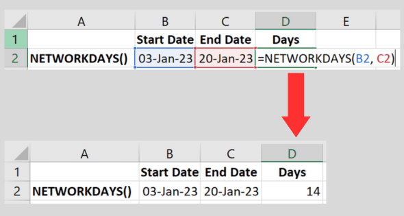
The NETWORKDAYS date function calculates the number of workdays between two dates. As this is working days, the calculation excludes weekends and specified holidays.
This is the format:
=NETWORKDAYS(Start, End, [Holidays])
The third parameter (Holidays) is optional. If you don’t use it, the formula will exclude weekends.
Follow these steps to use the simplest formula without specifying holidays:
- Enter the two dates in separate cells.
- In a new cell, type a formula like this:
=NETWORKDAYS(B2, C2) - Press enter.
Taking the dates I used in the previous example (3rd January and 20th January 2023), the result from this Excel function is 14.
This is three days less than using simple subtraction. That’s because there are two weekends during that timeframe (I double-checked).
Specifying holidays
You can give the formula a list of holidays to exclude in the calculation.
You do this by entering each holiday into a range of cells and put the range into the Holiday’s parameter.
That’s easier to understand with a worked example.
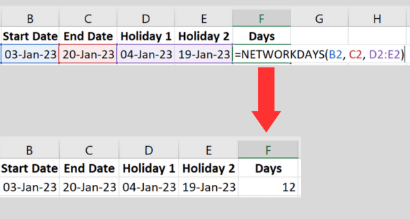
- The two dates are in cells B2 and C2.
- The first holiday date is in cell D2 and the second is in cell E2.
- In cell F2, use the formula:
=NETWORKDAYS(B2, C2, D2:E2) - Press the Enter key to see the result.
In our example, the result is 12. This is two days less than the previous calculation because the formula found the list of dates in the cell range we provided.
(I’m not showing cell A1 and A2 in the picture. Cell A1 is blank and A2 holds the description.).
By the way, if you have a long list of holiday dates and you’re not sure if it includes duplicates, the video below shows you how to check the data.
It also shows you how to remove the duplicates!
Specifying different days for weekends
Note that NETWORKDAYS uses Saturday and Sunday as the default weekend days for its calculation.
If your weekends are different, you can use the NETWORKDAYS.INTL function to customize the weekend day.
If you want to learn more about the format, here is Microsoft’s documentation.

The Older DATEDIF Function (Not Recommended)
You won’t find the DATEDIF function in the list of in-built functions in the current version of Microsoft Excel.
However, it still is possible to use it. Microsoft doesn’t list it because the company no longer supports the function except for special cases.
The problem is that it is not always accurate. That’s why I recommend that you avoid using this function.
I’ll describe it in case you are using an older version of the software. You may also find it in older templates you are working with. The syntax is:
=DATEDIF(Start, End, “d”)
Using “d” in the third parameter tells the function to calculate in days. Make sure to put the “d” in double quotes.
As an alternative usage, “m” does the calculation as the number of months, while “y” gives the number of years.
Here are the steps:
- Enter the two dates in adjacent cells.
- In a new cell, type a formula like this:
=DATEDIF(Start_Date, End_Date, "d"). - Press enter.
This will return the days between the two dates.
Using the cells in our previous examples, the function is: DATEDIF(B2, C2, “d”).
Unlike the other functions, this one shows the #NUM! error if the first date is after the second one.
Using The Current Date In Calculations
If you want one of the dates in the calculation to be the current date, Excel gives you the handy Today function.
You simply replace one of the cell references with TODAY(). In my worksheet, I’d only need column B to hold dates. Here is an example:
=DAYS(TODAY(), B2)
Somewhat confusingly, the equivalent function in VBA has a different name. Use the Date() function if you’re coding a macro.
How To Subtract Months Or Years To Find A Day
If you’re looking for the date from exactly one month ago, you may be tempted to subtract 30 days from the output of the TODAY() function.
However, this will only be accurate for a subset of months so it’s not a good method.
The EDATE function is for exactly this purpose. The syntax is:
=EDATE(start, months)
For my specific example of exactly one month ago, I would use:
=EDATE(Today(), -1)
This gives me the date a full month in the past. This is the best way to subtract months.
If you need to subtract years, the YEAR function calculates years from a given date.
What If The Start Date Is After The End Date?
If the first date is greater than the second, the recommended methods won’t see that as an error. They will do the calculation and provide a negative number.
For example, if I mistakenly switched the dates in the examples, the result is -17.
It’s always a good idea to prevent ourselves from making mistakes. You can use the IF function to check for an invalid date range and display an error message instead.
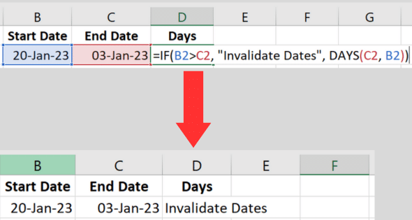
Here’s an example of how to incorporate the IF function with the DAYS function:
=IF(B2 > C2, "Invalid Dates", DAYS(B2, C2, "d"))
This Excel formula checks if the first date is greater than the second. If that’s the case, the “Invalidate Dates” text is displayed.
Otherwise, it will calculate the difference in days as before.
In the example below, I switched the two dates around. The function displays the text I specified for the IF() function.
Tips for Accurate Date Subtraction
When working with dates in Excel, it’s important to ensure accuracy in your calculations.
Here are my best tips to help you use date calculations.
Tip 1. Use the right formula
I recommend that you don’t use the DATEDIF() function. It is not always reliable.
Instead, choose one of the three other methods described in this article.
Tip 2. Format dates correctly
Make sure both the start and end date cells are formatted as dates.
To do this, follow these steps:
- right-click on the cell.
- select “Format Cells” (or press ctrl + 1 to open the dialog box).
- choose “Date” under the “Number” tab.
This will help avoid potential errors in your calculations.
Tip 3. Account for leap years
Be aware that leap years can influence how many days are between two dates.
Excel automatically accounts for leap years in its date calculations, so if you follow the correct formula and formatting, you should get accurate results.
You can find a list of leap years here.
Tip 4. Display the dates and results clearly
To improve the readability of your data and results, consider using some of Excel’s formatting features:
- Adjust column widths to accommodate the width of the content.
- Align date data in the center of each cell.
- Apply styles, such as bold or italics, to make column headers more distinct.
Common Errors and Troubleshooting

While working with dates in Excel, you might encounter a few common errors. Here are some troubleshooting tips to help you resolve these issues:
Error 1: #VALUE!
This error occurs when the cell values are not recognized as proper dates.
To fix this issue:
- Ensure both date cells are formatted as dates.
- Check your locale settings to interpret dates correctly.
Different locales have different date layouts (e.g., dd/mm/yy or mm/dd/yy).
Error 2: Incorrect results
If you’re obtaining incorrect results, consider the following
- Double-check how you entered your dates. Mixing up the month and day can cause calculation errors.
- Use network days if you only want to count working days between two dates by utilizing the NETWORKDAYS() function.
- Consistently use the same way of formatting dates throughout your worksheet to avoid confusion and errors.
- Avoid manual calculations by using the methods in this article.
Conclusion
In this article, we have explored various methods to subtract dates in Excel and calculate the difference in days between two dates.
By now, you should be confident in using the DAYS function, the NETWORKDAYS function, and simple subtraction to achieve accurate results.
Remember to always double-check your data, as incorrect or invalid formats may lead to unexpected outcomes.
When applying any of the methods discussed, ensure both the start date and end date are in the proper format so that Excel recognizes what they are.
Now that you are equipped with this knowledge, you can effectively track project durations, analyze trends, and manage deadlines, among other tasks.
Keep practicing and experimenting with different date formats and functions to harness the full potential of Excel’s date capabilities. Happy calculating!
Ready to take your Excel skills to the next level? Check out our Free Training!


