
Calculating a weighted average in Excel with percentages gives you the power to deal with data that has varying degrees of importance.
A weighted average is similar to the standard average, but it emphasizes specific values based on their assigned weights. When the different weights are expressed in percentages, the results are often more meaningful.
In this article, you will learn the steps to calculate a weighted average using percentages in Excel. We cover the necessary formulas, functions, and Excel tips that you need to know.

Let’s get into it.
What Is a Weighted Average?
Weighted averages and percentages are essential concepts in many fields, including finance, statistics, and data analysis.
A weighted average is a type of average that considers the relative significance of a set of values.
Let’s compare this to the simple average you have probably used many times. The simple arithmetic mean treats all values equally when calculating the result.
With a weighted average, not all values are of equal weight. The weights are assigned to values according to their importance or relevance.
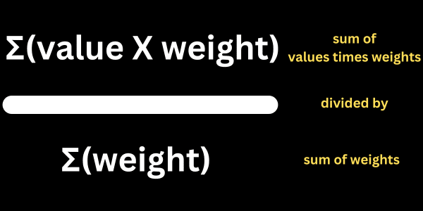
In mathematical terms, a weighted average is calculated by:

- multiplying each value with its corresponding weight
- summing the products to get the total
- dividing the total by the sum of the weights
The mathematical formula can be represented as:
Weighted Average = (?(value × weight)) / ?(weight)
You can write the mathematical formula when working with macros and VBA.
However, this tutorial uses a few helpful functions in Microsoft Excel to simplify the calculation. You’ll find that they are easy-to-use shortcuts.
Using Percentages Or Units
Some weighted calculations use percentages, and others use units.
For example, if you are averaging prices in a shop, you will be using monetary units that represent the price of an item.
If a pencil is fifty cents and a pen is a dollar, then the weights are 0.5 and 1.0, respectively.
College grades are more likely to be based on percentages. For example, the mid-term exam may be assigned 40% of the total grade, while 60% is assigned to the final exam.
This article focuses on calculating and displaying averages using percentages.
Setting Up Your Excel Worksheet
Before you calculate a weighted average in Excel, you need to set up your worksheet with the necessary data. Follow these steps:
- Input your data values in one column (e.g., Column B).
- Assign weights as a percentage in a separate column (e.g., Column C).
- Check that the weights add up to 100%.
This tutorial starts with an example from the world of sports. Coaches assess their players by different attributes, and some attributes are more valuable than others.
The coach decides on the percentage weight for each attribute and then scores the player. The weighted average gives a fuller picture of how the player measures up.
Copy this table into your Excel template:
| Attribute | Score | Percentage |
| Speed | 8 | 40% |
| Strength | 5 | 50% |
| Agility | 6 | 10% |
The weights above are represented as percentages, and their sum is 100%.
Formatting Cells for Percentages
For clarity, it’s essential to format the cells containing the weight values as percentages. Here are the step-by-step tasks:

- Select the weight cells that need to be formatted (e.g., Column B).
- Click on the “Home” tab in the Excel toolbar.
- Locate the “Number” group and click the “Percent Style” button (%). This will format the selected cells as percentages and display them with the % sign.
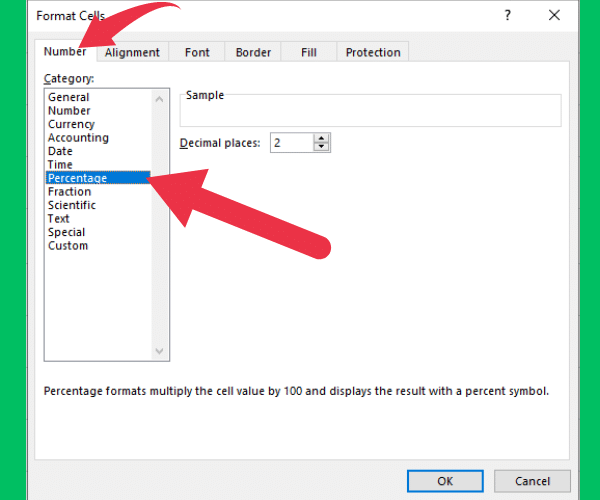
Upon completing these steps, your Excel worksheet should now be set up and ready for calculating the weighted average. Make sure your data and weight values are entered correctly and the cells containing the weights are formatted as percentages for improved readability.
How to Calculate a Weighted Average in Excel
The calculation of a weighted average involves a series of simple steps using the SUMPRODUCT and SUM functions.
These functions can be combined to find a final average value that takes into account varying importance or weights given to different values.
Using the Excel SUMPRODUCT Function
The Excel SUMPRODUCT formula is used to multiply two or more arrays of values and return the sum of their products.
An array refers to a list of values. The range of cells that contain the quantities is one array. The array that contains the price is a second array.
Dividing by the Total Weight
After using the SUMPRODUCT function to multiply and sum the item quantities and prices, you need to divide it by the sum of weights to calculate the weighted average.
Suppose the total weight represents the sum of quantities in column B.
By using the SUM function, like this: SUM(B2:B4), you will get the total weight.
This figure is used to divide into the result of the SUMPRODUCT result.
Instructions for Excel
Follow these steps in your Excel worksheet:
- Click on an empty cell, where the weighted average will be displayed.
- Enter the following formula: =SUMPRODUCT(B2:B4, C2:C4)/SUM(B2:B4)
- Press ‘Enter’.
Once you have completed these steps, Excel will display the weighted average price in the cell you selected.
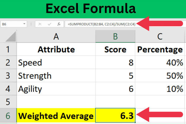
If you’re following this example, you may see a long number in the result cell with many decimal places.
At this point, you should tidy up the display by formatting the result cell to show two decimal places.
Breaking down the formula
Here’s a breakdown of the formula from the previous section:
- SUMPRODUCT(B2:B4, C2:C4) gets the sum of products of item quantities multiplied by their respective prices
- SUM(B2:B4) calculates the total weightage (sum of item quantities)
- SUMPRODUCT(B2:B4, C2:C4)/SUM(B2:B4) divides the sum of products by the total weight, providing the weighted average
Real-World Scenarios
Two common applications of this formula include grading systems and financial analysis.
These examples demonstrate how to apply weighted averages in Excel using percentages as weights.
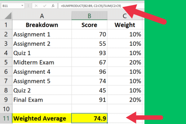
Grading Systems
When teachers and professors evaluate students’ performance in a course, they often use weighted averages to determine the final grade. In this case, each assignment, quiz, or exam has a specific weight or percentage contributing to the overall grade.
For instance, let’s assume the following grade breakdown:
- Assignments: 40% (total of 4, each worth 10%)
- Quizzes: 20% (total of 2, each worth 10%)
- Midterm Exam: 20%
- Final Exam: 20%
To follow the example, you can copy the data in this table into your spreadsheet. Put the first column in the table into column A.
| Breakdown | Score | Weight |
| Assignment 1 | 70 | 10% |
| Assignment 2 | 55 | 10% |
| Quiz 1 | 93 | 10% |
| Midterm Exam | 67 | 20% |
| Assignment 4 | 96 | 10% |
| Assignment 5 | 74 | 10% |
| Quiz 2 | 45 | 10% |
| Final Exam | 91 | 20% |
To calculate the weighted average in Excel, you can use the SUMPRODUCT function.

Assuming that the grades are in column B (from B2 to B9) and the corresponding weights expressed as percentages are in column C (from C2 to C9), the formula will look like this:
=SUMPRODUCT(B2:B9, C2:C9)/SUM(C2:C9)
This Excel formula calculates the weighted average using the provided grades and percentages.
Financial Analysis
Weighted averages also play an essential role in financial analysis, particularly when evaluating a stock portfolio’s performance. In such cases, the weight given to each stock can be based on the percentage of investment allocated.
Suppose you own the following stocks in your portfolio:
| Stock | Price | Shares | Investment (%) |
| Stock A | 100 | 5 | 30% |
| Stock B | 50 | 10 | 40% |
| Stock C | 80 | 3 | 30% |
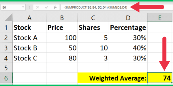
Assuming the stock prices are in column B (from B2 to B4), shares in column C (from C2 to C4), and the investment percentages in column D (from D2 to D4), the weighted average formula will be as follows:
=SUMPRODUCT(B2:B4, D2:D4)/SUM(D2:D4)
The above formula calculates the weighted average stock price based on the investment percentage for each stock. This value aids in assessing the portfolio’s overall performance.
This screenshot shows the calculation and results:
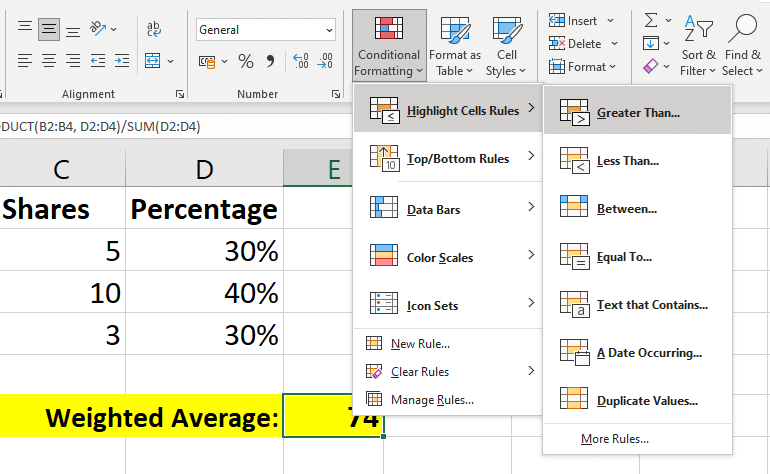
You can make your presentations even better by color-coding the values that fall above or below the weighted average. For example, higher values could be highlighted in green.
To do so, use conditional formatting to add a “highlight cell” rule with the “greater than” condition. This lets you specify the threshold and choose the highlight color.
Stock price analysis often combines the power of weighted averages with the frequency of closing prices in certain price ranges. Analysts assign weights to different price ranges and use Excel to create a frequency table that counts the times that a stock price fell into a price range over thirty days.
This allows the calculation of weight average daily closing prices based on the frequency. This helpful video shows you how to make frequency tables in Excel:
4 Common Mistakes and Troubleshooting
Here are the four most common mistakes you will encounter when calculating a weighted average in Excel.
1. Misaligned Data and Weights
Misaligned data and weights can also lead to inaccurate weighted average results. Accuracy is conditional on data and weights being aligned correctly in Excel.
The data should be listed in adjacent columns, with each value corresponding to its respective weight:
| Data (Column B) | Weights (Column C) |
| Value 1 | Weight 1 |
| Value 2 | Weight 2 |
If you notice that the data and weights are misaligned, adjust the columns in your spreadsheet to ensure a proper match between the values and their corresponding weights.
2. Not Accounting for Percentages
When dealing with percentages as weights, ensure that the weights are expressed as decimal values. For example, if a weight is represented as 20%, the decimal equivalent should be 0.20.
To convert a percentage to a decimal, divide the percentage by 100:
=C2 / 100
By accounting for percentages correctly, the weighted average calculation will yield accurate results.
3. Incorrect Cell References

It’s essential to ensure that the cell references are accurate. Incorrect cell references may lead to errors or inaccurate results in the calculation.
Check that the formulas include the appropriate cell ranges for both values and weights.
4. Using the wrong function
You’ve probably used Excel’s normal average function many times. This function isn’t used for weighted averages.
Standard deviation and the moving average are ways of capturing changes in data averages. Those calculations use different formulas.
The AVERAGEIF function lets you filter out values that don’t meet specific criteria. However, it’s better to assign the values a low percentage when calculating a weighted average.
Our Final Say
In this article, we have demonstrated the process of calculating weighted averages in Excel with percentages. Weighted averages provide valuable insights into data sets, highlighting the relative importance of a number of values.
Using the SUMPRODUCT function, Excel can easily calculate the weighted average by multiplying the corresponding data points and dividing the result by the total sum of the weights. The formula is as follows:
=SUMPRODUCT(data_range, weight_range) / SUM(weight_range)
This method is particularly useful when dealing with grades, survey results, or financial data, where some values carry more significance than others.
Mastering this technique can enhance data analysis capabilities, enabling users to make more informed decisions based on accurate and relevant data.
Ready to start building some strong Excel skills? Check out our Course on Excel.


