
Most Excel users think that the SUMPRODUCT function in Excel helps only to multiply the numbers in specified arrays and returns the sum of those products.
But, they are wrong.
By incorporating multiple criteria into the function, you can easily apply conditions on your data sets without having to go through the hassle of multiple calculations, conditional formulas, or even lengthy VBA codes.

Mastering the SUMPRODUCT function with multiple criteria can significantly enhance your data analysis workflows and make your reports more accurate and efficient.
To apply SUMPRODUCT with multiple criteria, you can use the below formula.
=SUMPRODUCT((array1 = criteria1) * (array2 = criteria2)*array3)When dealing with multiple criteria, the SUMPRODUCT function compares arrays and performs calculations based on the criteria you’ve set.
As you familiarize yourself with the SUMPRODUCT function and its various applications, you’ll quickly realize that this powerful feature is an essential tool in your data analysis arsenal.
Let’s get started.

Understanding SUMPRODUCT Function in Excel
The SUMPRODUCT function in Excel is a powerful and versatile tool that can handle multiple criteria calculations. It is particularly useful when you need to multiply ranges or arrays and then return the sum of those products.

You might find it handy for tasks that involve counting and summing data, similar to how COUNTIFS and SUMIFS functions operate.
To grasp the SUMPRODUCT function, it’s important to learn its syntax. The SUMPRODUCT syntax is as follows:
SUMPRODUCT(array1, [array2], [array3], ...)
Here, “array1” is the first range or array that you want to process, and “[array2], [array3], …” are optional additional arrays to include in the calculation. The function will multiply corresponding elements in each array and then sum the products.
In the table below, Column B displays the quantity, while Column C indicates the price for each product listed in Column A.
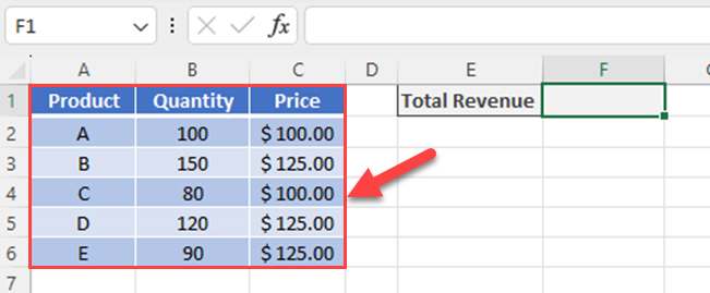
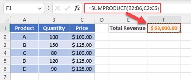
If you want to find the total revenue value, you can use the below SUMPRODUCT function.
=SUMPRODUCT(B2:B6,C2:C6)
SUMPRODUCT function can be used as an array formula as well.
For example, if you want to count the number of characters of an array, you can use the below formula.
=SUMPRODUCT(LEN(A1:A3))
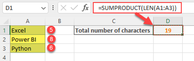
In this example, SUMPRODUCT helps to convert LEN function to array formula.
Now you know that SUMPRODUCT is a versatile Excel function used for multiplying corresponding values in multiple arrays and then summing the results.
It can also incorporate criteria to filter and perform calculations based on specific conditions within the arrays.
Application of Single Criteria in SUMPRODUCT
You can apply criteria when you want to do SUMPRODUCT calculations.
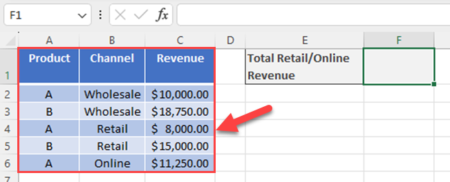
In the table below, Column B displays the channel, while Column C indicates the Revenue for each product listed in Column A.
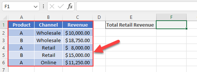
If you want to find the total retail revenue, you can use the below SUMPRODUCT function.

=SUMPRODUCT(C2:C6*(B2:B6=”Retail”))
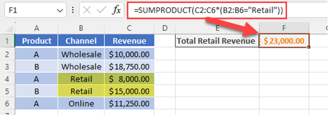
In the above example, the SUMPRODUCT function is like a SUM formula that can consider specific conditions, much like the SUMIF function.
Application of Multiple Criteria in SUMPRODUCT
This Excel function, SUMPRODUCT is especially useful when you need to work with data sets that have multiple conditions. In this section, we’ll explore how to apply multiple criteria using the SUMPRODUCT function.
When using the SUMPRODUCT function in Excel to work with multiple criteria, it’s essential to understand how logical operators, such as AND and OR, come into play.
These operators help you apply Boolean logic to your calculations, allowing for a more comprehensive and accurate analysis of your data.
AND Logic:
To apply AND logic in SUMPRODUCT, you can incorporate multiple conditions that all need to be met for the result to be true.
The SUMPRODUCT function multiplies the arrays together and sums the products only if all specified criteria match.
Here’s an example of how to use AND logic with SUMPRODUCT:
=SUMPRODUCT((array1="Criteria1") * (array2="Criteria2"), array3)
The formula above checks if the values in array 1 and array 2 match the respective criteria, and if both conditions are true, it multiplies the corresponding value in array 3.
In the table provided, Column B represents the channel, and Column C shows the Revenue for each product listed in Column A.
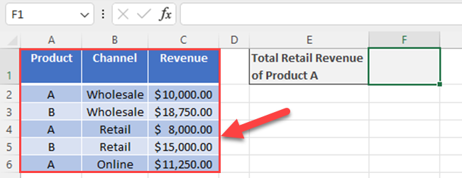
Now, if you want to calculate the total retail revenue of product A, you can use the below SUMPRODUCT formula.
=SUMPRODUCT(C2:C6*(B2:B6=”Retail”)*(A2:A6=”A”))
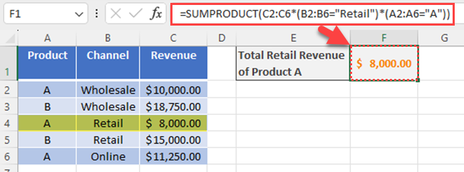
In this above example, Excel calculates a conditional sum in the Revenue (Sales) column. The first condition is Channel in column B should be “Retail”. The second condition is Product in the column A should be “A”. Then Excel SUM value only if both conditions are met.
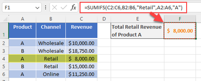
You can use the following formula using the SUMIFS function to get the same result.
=SUMIFS(C2:C6,B2:B6,”Retail”,A2:A6,”A”)
OR Logic:
Unlike AND logic, OR logic requires at least one condition to be true. In SUMPRODUCT, you can represent OR logic by adding (+) to the Boolean arrays instead of multiplying (*) as you do with AND logic.
An example of using OR logic with SUMPRODUCT is as follows:
=SUMPRODUCT((array1="Criteria1") + (array2="Criteria2"), array3)
In this case, the function will multiply the corresponding value in array 3 if either Criteria1 or Criteria2 is met.
In the table provided, Column B shows the channel, and Column C shows the Revenue for each product listed in Column A.
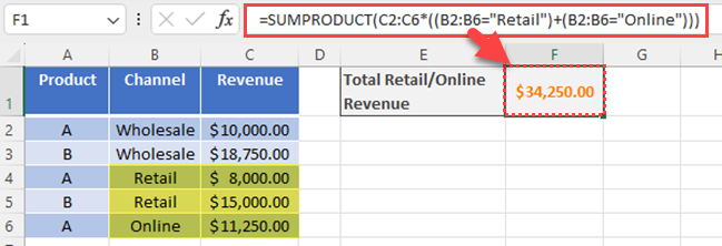
Now, if you want to calculate the total retail and online revenue, you have to use the SUMPRODUCT using the OR logic.

It means that you want to add revenue if the channel is Retail or Online. In other words, you have to apply both conditions in one column (Single array).
To calculate the total revenue (Total sales) of retail and online, you can use the below formula.
=SUMPRODUCT(C2:C6*((B2:B6=”Retail”)+(B2:B6=”Online”)))
What are Boolean Values in SUMPRODUCT?
In the previous examples, you have entered all arrays in the first array argument.
If you want to enter arrays separated with commas to the SUMPRODUCT formula, you have to convert true and false values to 1 and 0 (zero).
To work with Boolean (TRUE and FALSE) values within SUMPRODUCT, you can apply the double unary operator (–) to convert them into 1 and 0, respectively. This conversion allows you to perform arithmetic operations with the logical conditions.
The double unary (shows as –) operator can help in evaluating conditions, converting TRUE values to 1 and FALSE values to 0.
When using this operator within the SUMPRODUCT function, you perform logical tests on the arrays and multiply those results, ensuring only the conditions that meet your criteria are considered in the final calculation.
For example, applying the double unary operator within an AND logic SUMPRODUCT formula would look like this:
=SUMPRODUCT(--(array1="Criteria1"),--(array2="Criteria2"))
The following example shows how to apply double negative in SUMPRODUCT multiple criteria.
In the table provided, Column B represents the channel, and Column C shows the Revenue for each product listed in Column A.

Now, if you want to calculate the total retail revenue of product A, you can use the below SUMPRODUCT formula.
=SUMPRODUCT(C2:C6,–(B2:B6=”Retail”),–(A2:A6=”A”))
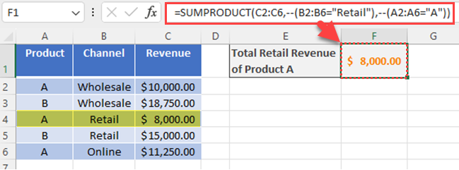
Using double negative, Excel converts logical values (True and false values) to 1 and 0 in each conditional array.
This method is especially useful for counting cells which are text cells.
Remember, when using SUMPRODUCT with multiple criteria, it’s crucial to use logical operators and understand their effects on your calculations.
Furthermore, correctly applying AND and OR logic, along with Boolean logic and the double unary operator, can greatly enhance the efficiency and accuracy of your Excel data analysis.
Using Arrays in SUMPRODUCT
When working with the SUMPRODUCT function in Excel, you’ll often deal with arrays. Arrays are continuous ranges of cells that contain values or data you want to process.
These arrays can be represented as array1, array2, array3, and so on, in the SUMPRODUCT function syntax: SUMPRODUCT(array1, [array2], [array3], …).
Keep in mind that when using arrays, Excel can handle a maximum of 255 arrays, and it’s essential to avoid discrepancies between rows and columns.
Additionally, be cautious when working with large arrays, as the complexity of the calculations might increase and affect your workbook’s performance.
In summary, using arrays in the SUMPRODUCT function allows you to apply multiple criteria and perform complex calculations.
Also, adopting a confident, knowledgeable, and clear approach while using the function in the second person point of view helps you create an effective, readable, and neutral-toned text in the English language.
But, what happens if you get errors?
Error Handling in SUMPRODUCT
When working with the SUMPRODUCT function in Excel, you may encounter Excel errors.
To effectively handle those errors, you need to understand the underlying causes and apply the appropriate solutions.
#VALUE! error typically arises when the arrays in your formula have a different number of rows and columns.
In other words, the #VALUE! error occurs when the SUMPRODUCT function has mismatched array dimensions. To resolve this issue, ensure that all arrays in your SUMPRODUCT formula have the same number of rows and columns (Same size).
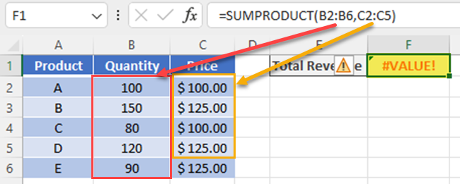
In the above example, you can see that the SUMPRODUCT formula has an error. The reason is arrays do not end in the same row.
To correct that you’ll need to adjust =SUMPRODUCT(B2:B6,C2:C5) to =SUMPRODUCT(B2:B6,C2:C6) so that both ranges have the same starting and ending row numbers.
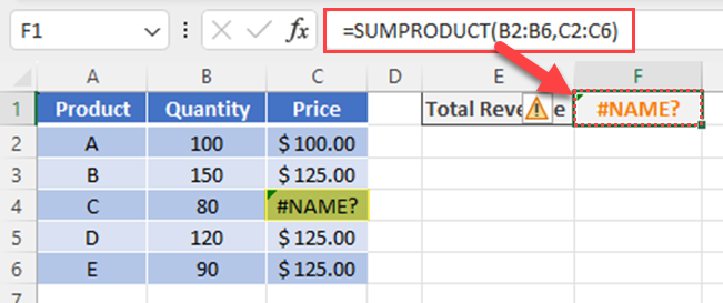
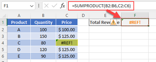
Another reason for encountering the #VALUE! error is having non-numeric values within the referenced range.
You’ll get an error for the SUMPRODUCT when cells contain an error.
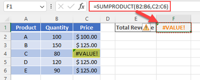
In summary, when utilizing the SUMPRODUCT function in Excel, be aware of potential #VALUE! errors that may occur due to mismatched array dimensions or non-numeric values within the referenced range.
Also, ensure that your formula adheres to the correct logic operations and thoroughly test it to avoid negative impacts on your analysis.
By paying close attention to error handling in SUMPRODUCT, you’ll be able to confidently perform calculations on your data and achieve accurate results.
Final Thoughts and Additional Resources
By now, you should be familiar with the powerful functionality of the SUMPRODUCT function in Excel, particularly in handling multiple criteria.
Using SUMPRODUCT allows you to streamline your calculations and accomplish tasks like counting and summing with multiple criteria more effectively.
Also, you have now acquired valuable knowledge about the SUMPRODUCT function and its many applications, allowing you to handle complex calculations and criteria in your spreadsheets more efficiently.
Keep practicing and expanding your Excel skills, and you’ll find even more ways to simplify your data analysis and make well-informed decisions.
If you like to learn the difference between SUM vs SUMX in Power BI, watch the video below.
Frequently Asked Questions
How to use SUMPRODUCT with multiple columns?
To use SUMPRODUCT with multiple columns, use the formula with criteria separated by asterisks, like this: =SUMPRODUCT((array1 = condition1)*(array2 = condition2)* array3). This formula evaluates conditions in different columns (arrays) and calculates the sum of corresponding values in a third column (array3).
What is the difference between SUMPRODUCT and SUMIFS?
SUMPRODUCT is a versatile function that works with arrays and can handle multiple criteria. It accepts various conditions and returns the sum of array elements that meet the given conditions. SUMIFS calculates the sum of cells that meet multiple criteria and is generally easier to use with simple criteria. However, SUMIFS is limited to working only with cell ranges, while SUMPRODUCT can work with arrays.
How to apply SUMPRODUCT with multiple arrays?
To apply SUMPRODUCT with multiple arrays, use a formula in this format: =SUMPRODUCT(array1* array2* array3). The function multiplies each element in array1 by the corresponding element in array2 and array3. Then, it adds the results to return the final sum.
What is the method for SUMPRODUCT and INDEX MATCH with several criteria?
To use SUMPRODUCT and INDEX MATCH with multiple criteria, follow these steps:
- Combine SUMPRODUCT with the Boolean logic, like this: =SUMPRODUCT((array1 = condition1)*(array2 = condition2) *row_number_array).
- Use the result in the INDEX function: =INDEX(return_array, MATCH(value, SUMPRODUCT_formula, 0)).
This method allows you to perform a more complex lookup based on multiple criteria.
How does SUMPRODUCT function with a single criterion?
When used with a single criterion, the SUMPRODUCT formula looks like this: =SUMPRODUCT((array1 = condition) * array2). This function evaluates the given condition in array1 and calculates the sum of corresponding elements in array2.
Are there limitations or advanced features of SUMPRODUCT in Excel?
SUMPRODUCT has some limitations and advanced features. It can handle a maximum of 255 arrays in Excel 365 and 2007, and 30 arrays in earlier versions. The function does not require the use of an array shortcut, making it more convenient for complex calculations with multiple criteria. However, if you need to work with a large number of arrays or require more advanced calculations, you may have to rely on other Excel functions or tools.


