How to Strikethrough Text in Excel? Easy Guide + Examples

Want to strikethrough some text in your Excel document but don’t know how?

Don’t worry, it’s easy, read on.

Keyboard shortcuts can be used to strikethrough text in Excel. On a PC, press “Ctrl + 5” or go to the “Home” tab, click on the “Font” group, and select the strikethrough icon.

On a Mac, use the shortcut “Command + Shift + X.” This feature allows you to edit cells to communicate changes without losing the original data.

But there are other great methods too.

In this article, we will show you step-by-step instructions on striking through text in Excel using different methods, such as keyboard shortcuts, the “Home” tab, and the “Format Cells” dialog box.

You will also learn how to strikethrough part of the text in the same cell and in a range of cells.

Let’s begin!

Prerequisites for Applying the Strikethrough Formatting

Before applying the formatting, you need to have the data spread throughout your document.

Here are the 3 basic steps to get you started:

1. Open a new Excel workbook or prepare an existing one for the desired data.
2. Enter the data into the spreadsheet.
3. Ensure the content is consistent and accurate before selecting the text to be formatted.

Now that you have the data ready, you can strikethrough text in Excel in several ways.

To select the text, left-click your mouse and drag the cursor over the words or numbers you want to apply the formatting to:

You’re now ready to strikethrough the text in the selected cell.

With a clear understanding of the basics, let’s dive into the detailed steps to apply strikethrough in Excel.

How to Apply Strikethrough In Excel

If you need to strikethrough text in Excel, you can use a few different methods.

In this section, we’ll cover how to apply strikethrough formatting to various cells using the Format Cells dialog box, the Home tab, and conditional formatting.

To strikethrough text in Excel, you can use the following methods for a range of cells:

• Format Cells dialog box: Select the range of cells, right-click, and choose “Format Cells.” Then, go to the “Font” tab and check the “Strikethrough” box under the “Effects” section.
• Home tab: Select the range of cells, go to the “Home” tab, and click the “Font” group’s “Strikethrough” button (S).
• Conditional formatting: Select the range of cells, go to the “Home” tab, and click “Conditional Formatting.” Then, select “New Rule” and choose “Format only cells that contain” with “Specific Text” and the proper formatting, including the strikethrough effect.

Let’s walk through these methods in detail.

Format Cells Dialog Box

To strikethrough text in a range of cells using the Format Cells dialog box:

1. Select the range of cells to which you want to apply the strikethrough formatting to.
2. Right-click within the selected range and choose “Format Cells…” from the context menu.
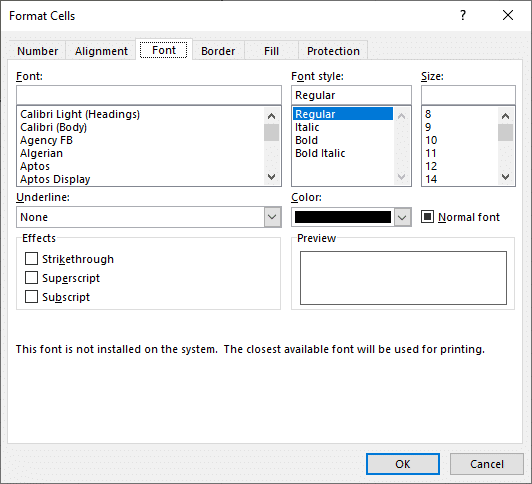
3. Navigate to the “Font” tab in the Format Cells dialog box.
4. Under the “Effects” section, check the “Strikethrough” box.
5. Click “OK” to apply the formatting to the selected range of cells.

Once you click “OK,” the text in the selected range will be formatted with a strikethrough line.

Having covered the Format Cells method, let’s now look at how to use the Home tab for strikethrough.

Perform Strikethrough Using the Home Tab

To strikethrough text in a range of cells using the Home tab:

1. Select the range of cells to which you want to apply the strikethrough formatting to.
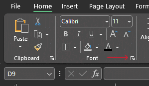
2. Go to the “Home” tab in the Excel ribbon.
3. Expand the font group and open up the formatting options.
4. In the “Font” group, click the “Strikethrough” button (S).

After clicking the “Strikethrough” button, the text in the selected range will be formatted with a strikethrough line.

Besides the Home tab, conditional formatting offers another powerful way to apply strikethrough based on specific conditions.

Conditional Formatting for Strikethrough

If you want to apply strikethrough formatting based on specific criteria within a range of cells, you can use conditional formatting to achieve this.

To set up conditional formatting for strikethrough, follow these steps:

1. Select the range of cells to which you want to apply conditional formatting to.
2. Go to the “Home” tab in the Excel ribbon.
3. In the “Styles” group, click “Conditional Formatting.”
4. Choose “New Rule” from the dropdown menu.
5. Select “Use a formula to determine which cells to format” in the “Select a Rule Type” section of the New Formatting Rule dialog box.
6. Enter the formula that will determine whether the strikethrough formatting should be applied. For example, if you want to strikethrough a cell containing the text “completed,” you can use the formula =SEARCH(“completed”, A1).
7. Click the “Format” button to open the Format Cells dialog box.
8. In the “Format Cells” dialog box, go to the “Font” tab and check the “Strikethrough” box under “Effects.”
9. Click “OK” to apply the conditional formatting.

Once you’ve applied conditional formatting with the strikethrough format, the cells that meet your specified criteria will display the formatting.

That’s how you apply the strikethrough formatting to the text in various cells.

In the next section, you will learn how to strikethrough part of the text in a cell without affecting the rest of the content.

After mastering whole cell formatting, let’s focus on how to strikethrough only part of the text in a single cell.

How to Strikethrough Part of the Text in a Single Cell

Strikethrough formatting can be applied partially in Excel. To apply the strikethrough style on a specific part of the text in a cell:

1. Click on the cell that contains the text you want to format.
2. Press F2 or double-click on the cell to enter the edit mode.
3. Use the arrow keys to navigate to the portion of the text you want to format with the strikethrough style.
4. Highlight the characters by holding the Shift key and pressing the arrow keys.
5. Apply the strikethrough formatting by using the previously mentioned techniques.

To open the “Font” dialog box in Excel, press Ctrl + Shift + F while selecting the desired range of cells. You can then easily apply the strikethrough style to parts of the text in the selected cells.

Remember, these formatting options can lead to a cluttered visual presentation. Be mindful when applying them to your data.

To enhance efficiency, let’s switch gears and explore various keyboard shortcuts for applying strikethrough in Excel.

6. Keyboard Shortcuts for Strikethrough in Excel

When working with a strikethrough in Excel, keyboard shortcuts can help you save time and make your workflow more efficient.

Action	Shortcut (Windows)	Shortcut (Mac)	Notes
Apply Strikethrough	Ctrl + 5	Command + Shift + X	Directly applies/removes strikethrough formatting.
Open Format Cells Dialog	Ctrl + 1	Command + 1	Opens the Format Cells dialog box where you can select strikethrough under the Font tab.
Access Ribbon Commands	Alt (then follow key tips)	Control + Option (then follow key tips)	Enables key tips on the ribbon for further keyboard navigation.
Apply Strikethrough from Home Tab	Alt + H + 4	Control + Option + H (then select Strikethrough)	Specific for Excel versions where this shortcut is applicable. Might vary based on Excel version and settings.

Excel provides various keyboard shortcuts for everyday tasks, including applying strikethrough to text. These shortcuts can be handy for users who frequently use this feature in their work.

The strikethrough shortcut in Excel has a unique identifier or mnemonic, an underlined character. It’s easy to apply this formatting by pressing Ctrl + 5.

If you are using a Mac, the shortcut for strikethrough is Command + Shift + X.

To apply the strikethrough formatting using the ribbon and the strikethrough icon, you can also use the keyboard shortcut method by pressing the following keys:

1. Press the “Alt” key to display the shortcut key tips on the ribbon.
2. Press the shortcut key for the desired tab.
3. Press the shortcut key for the specific command.
4. Release the “Alt” key once you’ve pressed the necessary keys.

For example, to apply the strikethrough formatting on the “Home” tab, press Alt + H + 4. However, this method may vary depending on your Excel version and settings.

The “Format Cells” dialog box has multiple keyboard shortcuts to speed up the formatting process. You can use them to navigate between tabs, apply changes, and confirm your preferences.

For example, to apply the strikethrough formatting, press Alt + O, and then press Alt + K to check the strikethrough box. Remember, these shortcuts should be combined with the appropriate key tips for the most efficient formatting.

Using these keyboard shortcuts, you can easily apply the strikethrough effect to the relevant cells. It will help you save time and streamline your workflow when working with formatted data.

Armed with these shortcuts, let’s delve into some tips for effectively working with strikethrough in Excel.

6 Top Tips on Working with Strikethrough In Excel

1. Strategic Application: Use strikethrough judiciously to avoid cluttering your spreadsheet. Overuse can render your data challenging to interpret.
2. Uniformity is Key: Ensure consistency in applying strikethrough across your spreadsheet to maintain a coherent presentation.
3. Differential Signaling: Experiment with varying colors or line weights for strikethrough to signify different stages of task completion or to highlight varying degrees of importance.
4. Synergistic Formatting: Combine strikethrough with other formatting tools like bold or italic fonts. This not only enhances visual appeal but also aids in organizing information more effectively.
5. Indicating Evolution: Strikethrough is particularly effective in denoting updates or modifications in your data. For instance, applying strikethrough to discontinued items in a product inventory keeps them in the record for reference while clearly marking their status.
6. Integration with Excel Functions: Strikethrough can be dynamically applied using Excel’s formulas and functions. For example, employing the IF function to automatically strike through a cell when a certain criterion is fulfilled, such as completing a task, streamlines data management and enhances clarity.

These techniques improve the visual management of your spreadsheets and enhance the efficiency and clarity of your data representation.

As we wrap up, let’s summarize the key points for applying strikethrough effectively.

Final Thoughts

Microsoft Excel provides several quick and easy methods to apply strikethrough formatting to data, helping you effectively communicate revisions and track changes.

The strikethrough effect is beneficial when working with spreadsheets and can be applied using keyboard shortcuts, the ribbon, or conditional formatting. You can also strikethrough text in a single cell or a range of cells in your worksheet.

Remember, you can combine the strikethrough formatting with bold, italics, and other cell formatting options for enhanced clarity and readability.

Excel also offers the flexibility of applying strikethrough to specific portions of text within a cell.

Moreover, the keyboard shortcuts for strikethrough make applying the desired effect to your data quick and easy.

Do you want to learn more about supercharging your Power BI workflow? Check out the EnterpriseDNA Youtube Channel.

Frequently Asked Questions

Having covered the essentials, let’s address some frequently asked questions to further clarify your understanding of strikethrough in Excel.

How to remove strikethrough in Excel?

You can use keyboard shortcuts to remove strikethrough from selected text or cells.

For Windows, press Ctrl + 5 to apply or remove the formatting.

On Mac, use Command + Shift + X.

You can also apply or remove the formatting from the Format Cells dialog box on the Home tab of the ribbon.

How to add a strikethrough in Excel for a single cell?

First, select the cell to apply strikethrough to the content within a single cell.

Then, use the keyboard shortcuts Ctrl + 5 (Windows) or Command + Shift + X (Mac).

Alternatively, go to the Home tab -> Font group, and click the Strikethrough button (it looks like “ab” with a line through it).

How to add a strikethrough in Excel for multiple cells (or a range)?

To add strikethrough formatting to multiple cells or a range, follow these steps:

1. Select the cells or range where you want to apply the formatting.
2. Use the keyboard shortcuts Ctrl + 5 (Windows) or Command + Shift + X (Mac) to toggle strikethrough on or off.

You can also access strikethrough from the Format Cells dialog box: select the cells or range, then right-click and choose Format Cells.

Go to the Font tab in the dialog box and check the Strikethrough option under Effects.

How to cross out text in Excel?

Strikethrough formatting is used to create a horizontal line through the middle of the text in Excel, often described as “crossing out” the text.

To apply strikethrough, use the keyboard shortcuts Ctrl + 5 (Windows) or Command + Shift + X (Mac) on a selected cell or range of cells.

Alternatively, you can access the Strikethrough button from the ribbon Home tab -> Font group.

What is the strikethrough hotkey (or keyboard shortcut)?

The keyboard shortcut to apply or remove strikethrough formatting in Excel is Ctrl + 5 for Windows. On Mac, use Command + Shift + X.

These shortcuts can quickly toggle the strikethrough effect on or off for the selected cells or text.

How to strikethrough in Google Sheets?

The method for strikethrough formatting in Google Sheets is similar to Excel.

Select the cell(s) or range where you want to apply strikethrough, then use the keyboard shortcuts Ctrl + Alt + Shift + 5 (Windows) or Command + Option + Shift + X (Mac).

You can also access this command from the toolbar: go to Format -> Text -> Strikethrough. This will apply the strikethrough effect to the selected content in the corresponding cells.