
Knowing how to alternate colors in Excel can be a game-changer; there’s little more satisfying than a well-organized and visually straightforward spreadsheet.
Well, that’s what we think!
So, how do you alternate colors?

Simple.
To get started, you can follow these steps:
Select the range of cells where you want to apply the color scheme.
Navigate to the “Home” tab on Excel’s ribbon.
Go to the “Styles” group and click the “Conditional Formatting” option.
Choose the “New Rule” option under the “Conditional Formatting Rules Manager” dialog box.
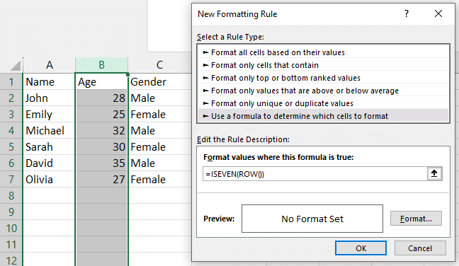
Select the “Use a formula to determine which cells to format” rule.
Input the formula and select the formatting options, such as fill color, font color, etc.
Click OK to apply the alternating color scheme on Excel.
By organizing your data with alternating colors in Excel, you’ll be able to produce visually appealing and effective spreadsheets.
In this article, we will show you the 3 best ways to get your spreadsheets looking awesome.
Let’s get into it!
7 Major Benefits of Using Alternating Colors in Excel Tables

Let’s look at the 7 major benefits of using alternating colors in Excel.

Reduces Errors: Alternating colors help prevent data entry and analysis mistakes by making it easier to follow rows.
Facilitates Comparisons: It is easier to spot trends and patterns and compare data across rows.
Improves Accessibility: Helps individuals with visual impairments or dyslexia by separating rows clearly.
Reduces Eye Strain: Breaks up the monotony, aiding focus and minimizing eye fatigue during prolonged data review.
Customization and Emphasis: Allow for personalization and highlighting important data, aligning with branding or specific color coding.
Facilitates Data Segmentation: Useful for visually separating and distinguishing different data groups or categories.
Enhances Presentation: Makes tables in reports or presentations more engaging and easier for audiences to understand. This makes the data more visually appealing, too.
Next, let’s see how we can apply alternating colors to tables.
3 Best Ways to Apply Alternating Colors in Excel

1. Use conditional formatting rules
To apply alternating colors in Excel, select the range of cells you want to arrange in a Microsoft Excel worksheet.
Navigate to the “Home” tab on the ribbon interface and go to the “Styles” group.
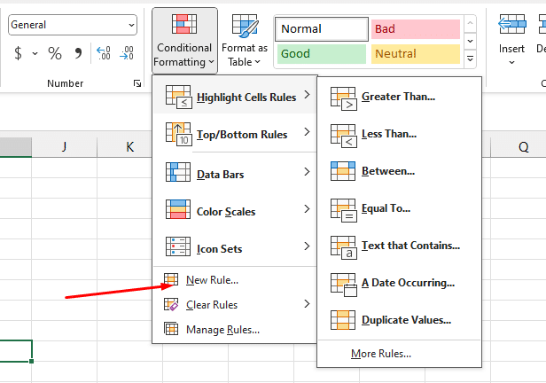
Click on the “Conditional Formatting” option, and in the dropdown menu, choose “New Rule” to open the “New Formatting Rule” dialog box to apply a conditional formatting rule to your data.
If the New Formatting Rule dialog box does not open, click “Conditional Formatting” and select New Rule from there.
In the New Formatting Rule dialog box, you’ll have to define a formula to determine which cells will be formatted based on specific criteria.
You can also choose from several formatting options, such as cell fill color, font color, font styles, etc.
For example, the ‘Use a formula to determine which cells to format’ rule will bring up a ‘Format values where this formula is true’ field, where you’ll input your formula.
The formula will depend on your data and the Formatting you want to apply. Alternatively, you can use the inbuilt formulas by selecting the inbuilt formulas from the ‘Select a Rule Type’ box.
The formula will look like “=ISEVEN(row())” where “row() ‘s function is used in Excel to return the current row number of a cell when it was when defining the format condition.
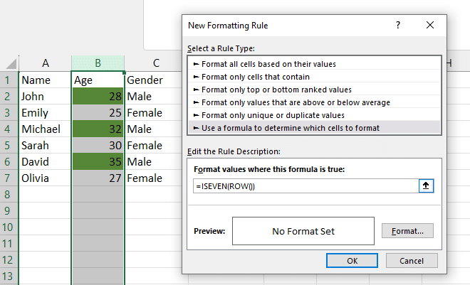
After inputting the formula, click on the Format button to bring up the ‘Format Cells’ dialog box, where you can choose cell formatting options like the fill color, font color, borders, etc., to apply the green and white color scheme and click on the OK.
In the “New Formatting Rule” dialog box, click OK. Based on your defined rules, the alternating color arrangement will be applied to the selected range of cells.
While the two-color scheme example is given above, Excel provides a variety of images, text styles, and templates to help you get the starting alternating color layout right.
You can choose from seven pre-designed color components and a ‘New rule’ option, allowing you to create custom table color schemes that automatically calculate when rows are added or deleted.
Similarly, highlight your alternate rows and cells as desired by selecting the cell or range and applying a conditional format.

Next, let’s look at how to do banded colors by applying a table style.
2: Using Table Styles
Now, as you select the column, click on the ‘Format as Table’ feature within the Home tab under the styles in “Excel 2007-2010” and under the ‘Styles’ group of the Excel ribbon interface in 2012 and later versions.
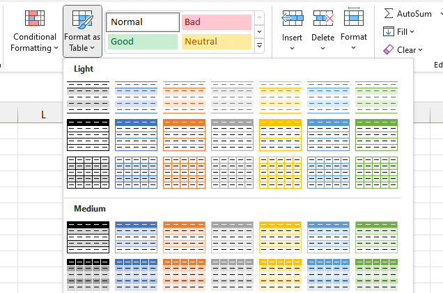
You can also use the shortcut for this method: press Ctrl + T. A listing of different row table styles will appear on the display screen.
Therefore, select the one you want by scrolling, and Excel will automatically assign the selected style to the range of cells.
If you want to apply alternating colors to a large dataset, you can use VBA.
3: Using VBA Codes (Visual Basic for Applications)
As mentioned above, applying this technique manually becomes tiresome when dealing with large data sets.
You can speed up this process using VBA (Visual Basic for Applications) codes.
The provided code below can add a custom alternating row color (i.e., zebra striping) in an Excel table, making it easy to follow the data across the spreadsheet.
1. Open the Visual Basic for Applications (VBA) editor by pressing Alt + F11 or find it in the developer tab.
2. In the editor, click “Insert” and “Module” to create a new module.
3. Paste the following VBA code into the module:
Paste the VBA Code: In the new module window, paste the VBA code you want. It might look something like this:
Sub AlternateRowColors()
    Dim MyTable As ListObject
    Dim i As Long
    Dim Color1 As Long
    Dim Color2 As Long

    Set MyTable = ThisWorkbook.Worksheets("Sheet1").ListObjects("MyTable")
    Color1 = RGB(240, 240, 240) ' Light grey color
    Color2 = RGB(255, 255, 255) ' White color

    For i = 1 To MyTable.ListRows.Count
        If i Mod 2 = 0 Then
            MyTable.ListRows(i).Range.Interior.Color = Color1
        Else
            MyTable.ListRows(i).Range.Interior.Color = Color2
        End If
    Next i
End Sub
To use this VBA code, you’ll need to follow these steps:
Change MyTable to the name of your table.
Change RGB(240, 240, 240)to the RGB color code of your desired row banding color.
Run the macro by clicking the “Run” button or pressing F5. Once executed, the VBA code will apply the alternating row colors to the entire table using a specified color selected using the RGB color model (i.e., the RGB function).
Do you want to maximize your efficiency in applying alternate row colors? Read on below.
Maximizing Efficiency with Alternating Row Colors in Excel

When dealing with large datasets or multiple worksheets in Excel, time is of the essence. You don’t want to get bogged down in the tedious task of manually formatting each row. Here’s how to speed up the process and make your life easier:
Leverage the Fill Handle: This is a great tool for quickly applying Formatting across multiple rows. Just drag the Fill Handle across the rows you want to format, and Excel will do the rest.
Utilize Format Painter: If you’ve got the perfect Formatting on one worksheet and want to replicate it on others, the Format Painter tool is your best friend. Copy the Formatting from one worksheet and paste it onto another with a few clicks.
Create a Custom Table Style: This is a real-time save for future projects. Once you’ve set up a formatting style that works for you, save it as a Table Style. Next time, you can apply it with just a click.
Implement Conditional Formatting: This feature adds a layer of intelligence to your Formatting. Set up rules to alternate row colors based on specific criteria, like values in a particular column or the presence of specific text or numbers in a cell.
Excel’s built-in table feature streamlines the process of applying alternating row colors. Select your data range and hit the “Format as Table” button in the Home tab.
You can choose from various table styles that include alternating row colors and customize them to suit your preferences.
Are you running into issues trying to apply alternate row colors?
Troubleshooting Issues When Applying Alternating Colors

Hey there! Are you struggling with alternating row colors in your Excel tables? Let’s dive into some common issues and how to fix them.
Firstly, are your banded rows not showing up?

This might be because the Banded Rows option isn’t enabled. Go to the Table Design tab and ensure it’s checked. If you’re using a custom table style, make sure it’s set to display banded rows.
Are you encountering inconsistent row coloring?
This often happens if you’ve manually formatted some cells, which can override the table style. You can remove this manual Formatting or tweak your table style to include these changes.
Do your alternating row colors disappear after sorting or filtering?
Excel sometimes struggles with rendering. Refresh your table by toggling the Banded Rows option or reapply your style.
Do you want to apply alternate row colors to a non-table range?
Conditional Formatting is your friend. Use a formula like =MOD(ROW(),2)=0 to color every other row.
Are you having issues with row colors not showing in your printed document?
Check your print settings. They must include background colors and images for your alternating colors to print.
Are the row colors affecting the readability of your text?
The trick is in the color choice. Go for lighter shades for your alternating rows to keep your text legible.
Only part of your table showing alternate colors?
Ensure you select the entire table when applying or changing your table style. Partial selections can lead to uneven coloring.
Need different colors for specific rows?
Banded Rows might not suffice. Instead, use Conditional Formatting with specific rules for those rows.
Mixing up banded rows with banded columns?
Remember, banded rows color alternate rows, while banded columns color alternate columns. They serve different purposes.
Using an older version of Excel and facing issues with this feature?
These features have improved over time. Upgrading to a newer version of Excel or using conditional Formatting can be a good workaround.
Here are a couple more tips: To create a custom table style with your preferred alternating row colors, head to the Table Design tab, click “New Table Style,” and set it up. Also, apply these colors only where necessary to keep your worksheet tidy.
Staying updated with Excel ensures you access the latest features and improvements.
Let’s wrap this up by reflecting on some final points.
Final Thoughts

Perfecting your table’s visual representation by setting up an alternating color scheme may seem simple, but it’s easy to bring more clarity to the data at hand.
It will help your readers to pinpoint those significant values and their corresponding categories at a glance. This, in turn, can facilitate faster decision-making.
With these simple tricks, creating visually appealing tables will lead you to more straightforward and practical data analysis. Happy Excel-ing!
Do you want to learn more about referencing vs duplicating queries? Checkout this great explanation on EnterpriseDNA’s YouTube channel:
Frequently Asked Questions

How do I format alternate rows in a pivot table?
To format alternate rows in a pivot table, you can use the built-in table design features or apply conditional Formatting manually.
For the latter, use the “MOD” function in a new column of your data and apply conditional Formatting based on the results.
Can you set up conditional Formatting to alternate every other row based on values in a column?
Yes, you can set up conditional Formatting to alternate every other row based on values in a column.
Choose “Use a formula to determine which cells to format” when setting up the rule, and use the “MOD,” “ISEVEN,” and “ISODD” functions in your formula to achieve the alternating effect.
How can I change the row colors in a long table automatically?
To change row colors in a long table automatically, you can set up conditional Formatting with a formula that adjusts the row color based on the current row number, such as “=ISEVEN(ROW())” for even rows and “=ISODD(ROW())” for odd rows.
This will ensure that the colors will continue to alternate as more rows are added to the table.
Is it possible to make the rows change color automatically based on the cell content?
Yes, you can make the rows change color automatically based on the cell content.
Use conditional formatting rules with formulas referencing the cell content and apply the desired color formatting.
How can I fill colors in alternate cells in the table?
To fill colors in alternate cells in a table, you can use conditional Formatting with a simple formula such as “=MOD(ROW(), 2) = 0” for even rows and “=MOD(ROW(), 2) = 1” for odd rows.
Apply the desired cell fill color, and Excel will automatically fill alternate cells based on the condition.
What’s the best practice for alternating row colors on a table?
A best practice for applying an alternating row color to a table is using Excel’s built-in table formatting features, found under the “Design” tab in the table tools.
Choose one of the predefined table styles or customize it for your needs. Alternatively, you can use conditional Formatting and adjust the row colors based on the row number or other conditions.
How do I apply shading to alternate rows in a table using conditional Formatting?
To apply shading to alternate rows in a table using conditional Formatting, follow these steps:
Select the range of cells in your table where you want to apply the shading.
Go to the ‘Home’ tab, and click ‘Conditional Formatting’ in the ‘Styles’ group.
Choose ‘New Rule’ from the dropdown menu.
In the New Formatting Rule dialog box, select ‘Use a formula to determine which cells to format.’
Enter the formula =MOD(ROW()-ROW(first_cell_reference), 2) = 0, where first_cell_reference is the reference of the first cell in your selected range. This formula will identify alternate rows starting from the first cell of your selection.
Click the ‘Format’ button, choose your desired shading color under the ‘Fill’ tab, and click ‘OK.’
Click ‘OK’ again in the New Formatting Rule dialog box to apply the shading to alternate rows.
This method will shade alternate rows in your table, enhancing readability and visual appeal.


