
Sorting data in Excel is a crucial skill when managing your information. One challenge you may encounter is keeping rows together while sorting, ensuring that related data stays linked when organizing your spreadsheet by a particular column.
The most common method to sort data with two or more columns in Excel while keeping rows together is to choose “expand the selection” in the sort dialog box. There are other methods, including the use of the sort function and custom lists.
You will learn all these methods in this article by walking through multiple scenarios.

How To Sort While Keeping Rows Together
Before we dive into the techniques, let’s take a look at the problem you want to avoid.
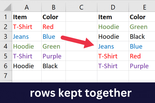
Suppose you have inventory data of clothing apparel where the type of item is in column A and the color is in column B. This is the data:
T-Shirt, Red
Jeans, Blue
Hoodie, Green
T-Shirt, Purple
Hoodie, Black
You want to sort the items in alphabetical order while keeping the association between the item and its color. This is what the sorted rows should look like (I’ve color-coded the fonts to make it clearer):
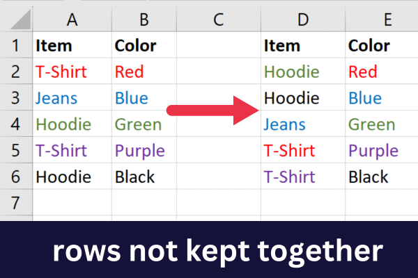
If you only sort the first column, the colors won’t move with their associated item. This will lead to jumbled data which loses all meaning.
Here are the results of an incorrect sorting method:
Now that you’re clear on what you want to achieve, let’s look at how to access Excel’s sort options.

3 Ways to Access The Sort Commands
The most common way to sort in Excel is to use the Sort command. There are three ways to access this feature:
Home tab
Data tab
Right-click
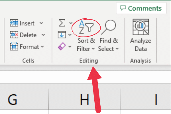
The Home Tab
Go to the Home tab.
Expand the “Sort & Filter” drop-down menu in the Editing group.
Choose the ascending or descending order option.
Excel assumes that you have a header row with this option.
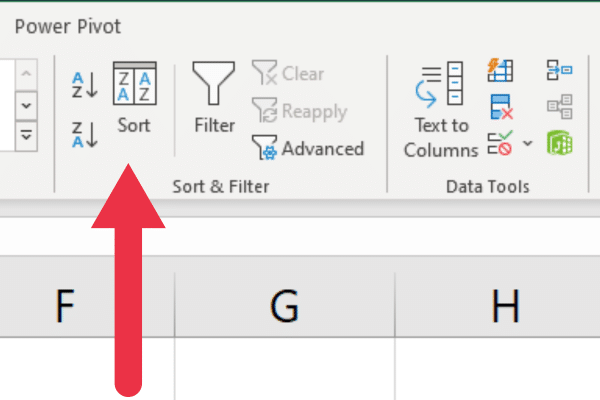
The Data Tab
Go to the Data tab.
Click on the Sort button in the Sort & Filter group.
Choose your sort options in the sort dialog box.
This method allows you to specify if your data has column headers.
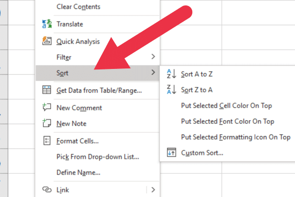
Right-Click
Select the data you want to sort.
Right-click.
Choose “Sort” from the drop-down menu (near the bottom).
How to Sort By Selecting Multiple Columns to Keep Rows Together
This method works when you want to sort by the first column in the data set. If the target column is not column A, then use one of the other methods in this article.
To use this method, you will select all the data involved before using the Sort command. This means that you are not simply selecting one column.
In our sample data above, you would either select the entire worksheet, the specific data range of cells from A1 to B6, or the two columns A and B.
Follow these steps:
Select all the cells that are related (or Ctrl-A for everything).
Go to the Home tab.
Expand the Sort & Filter drop-down.
Choose “Sort A to Z”.
Note that you won’t see extra prompts about how you want to sort the data. Microsoft Excel assumes that you want to keep associated rows together because you selected all the data.
If you have a header row, it will also be recognized.
How to Sort With Excel Prompt to Keep Rows Together
In the previous section, you ensured that your sort request was unambiguous by selecting all the data you wanted to include.
However, you may wish to sort by a column that is not the first in the worksheet. For example, suppose you want to sort the sample data by the color of the garments.
Follow these steps:
Select the column you want to sort by clicking on its header letter.
Go to the Home tab.
Expand the Sort & Filter drop-down.
Choose “Sort A to Z” (or your preference).
In the “Sort Warning” window that appears, choose “Expand the selection”.
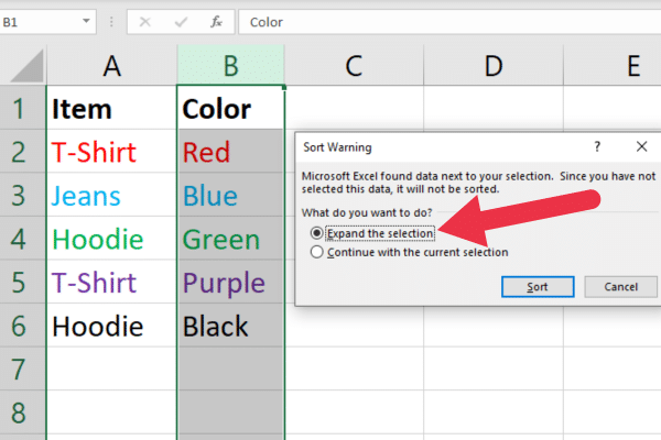
Note that Excel detected that there were columns adjacent to the one that you selected. In this scenario, Excel asks you whether you want to include multiple columns are not.
By expanding the selection, Excel sorts the chosen column while keeping the associated data in the same row intact.
How to Use The Sort Function to Keep Rows Together
The SORT function in Excel automatically keeps rows together when sorting.

This function is particularly useful because you can use it in a formula and it automatically updates when your data changes.
The SORT function is a dynamic array function. If you enter it into a single cell, Excel will automatically fill in the other cells needed to display the full range of sorted data, provided there are enough blank cells available.
After entering this formula in a cell, Excel will display the sorted version of your data starting from that cell. Note that this won’t change the original data; it will just display a sorted version of it.
The syntax of the SORT function is this:
=SORT(array, [sort_index], [sort_order], [column_or_row]
array: the range of cells to sort by.
sort_index: the column to sort by.
sort_order: TRUE for ascending (the default), and FALSE for descending.
column_or_row: FALSE for columns (default), and TRUE for rows
Let’s say you have data in cells A1 through B6 with a header. You want to sort this data by the values in column A in ascending order. Use this formula:
=SORT(A2:B6)
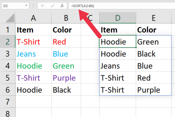
Be careful not to include the cell with the function in the array. Otherwise, you will have a circular reference.
Sorting And Filtering Together
The FILTER function in Excel is used to filter a range of data based on certain criteria, rather than to sort data. However, you can combine the FILTER function with the SORT function to both filter and sort data while keeping rows together.
The FILTER function is also a dynamic array function (like SORT). As I mentioned in the previous section, Excel will fill in the other cells needed to display the full range of filtered data.
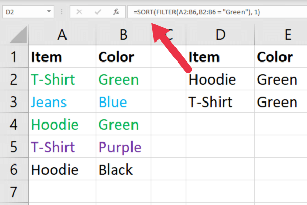
Suppose that some of the clothing items in the sample data have the same color. You want to arrange the data to show red garments sorted alphabetically. This requires two steps:
Filter the rows on column B (color).
Sort the filtered rows by column A (name of item).
This is the syntax of the FILTER function:
=FILTER(array, criteria, [if_empty])
array: the range of cells to sort by.
criteria: what to filter by.
if_empty: what to return if there is no match.
The key is to wrap the SORT function around the filtered results. For our example, you’d use this formula:
=SORT(FILTER(A2:B6,B2:B6 = “Green”), 1)
After entering this formula in a cell, Excel will display the filtered and sorted version of your data starting from that cell. Note that this won’t change the original data; it will just display a filtered and sorted version of it.
How to Use Custom Lists to Sort And Keep Rows Together
Custom lists in Microsoft Excel allow you to define your own sorting rules based on specific items. This is useful when you encounter a dataset where the default alphabetical or numerical sorting is not suitable.
Suppose you want to sort items so that purple is always before red which is always before blue etc. You can set up a list of colors in the precise order that you want.
There are two stages to ordering by a custom list:
Create the list.
Use the list as an order sequence.
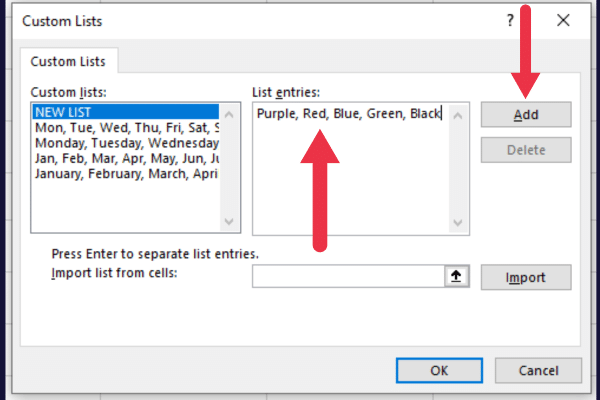
How to Create The Custom List
Go to the File tab.
Choose Options.
Click on Advanced.
Scroll down to the General section.
Click Edit Custom List to open the Custom Lists Dialog Box.
Add your ordered entries as a comma-delimited list.
This picture shows a list of colors typed into the interface.

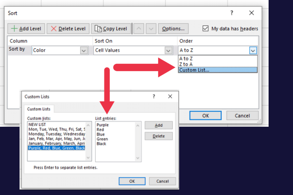
How to Use The List
Now that you’ve created your list, you can apply it to a set of data.
Select the column you want to sort by.
Go to the Data tab.
Click on the Sort button in the Sort & Filter group.
Choose “expand the selection” to view the sort dialog box.
Expand the drop-down list under the “Order” title.
Choose “Custom List”.
Choose your list.
Click OK twice.
This infographic shows the sequence:
3 Tips For Handling Data Types
When dealing with various data types in Excel, such as text, day, month, and last name, it’s essential to be aware of their distinctions. To achieve accurate sorting results, follow these tips:
For text sorting (alphabetical order), select a cell in the column you want to sort, go to the Data tab, and click either Sort A to Z (ascending) or Sort Z to A (descending).
When sorting by day or month, ensure your dates are in a consistent format (e.g., MM/DD/YYYY).
If sorting by age or numbers, make sure all data in the column is stored as the same type (text or numbers).
4 Tips For Efficient Sorting
Here are our best tips for efficient sorting:
If there are hidden columns or hidden rows in your data, unhide them before sorting.
It’s helpful to use the Freeze Panes feature when sorting lengthy data.
You can ensure that the sorting order isn’t changed by locking the cells.
Remember that blank rows will be pushed to the end when sorting i.e. eliminated.
Sorting data to eliminate blank rows is useful preparation when you’re looking for distinct values in your data. This video shows the task in action:
Final Thoughts
Sorting is one of the most common tasks when working with an Excel spreadsheet.
You have learned how to sort alphabetically or numerically in ascending or descending order while keeping rows intact.
This ensures that the meaning of your data is kept intact and further data analysis is accurate.


