Errors in Excel are a pain and seeing those green triangles representing errors is downright annoying, luckily Excel has 5 great ways to manage and suppress them.
To ignore all errors in Excel, you can disable the background error-checking feature globally. Go to File > Options > Formulas, and under “Error Checking,” uncheck “Enable background error checking.” This method is quick and comprehensive but should be used cautiously to ensure important errors are not overlooked.
In this article, we will go over all the top ways how to ignore all errors in Excel.
We’ll show you the 5 top methods of error removal including formatting cells as text, selecting and ignoring errors in bulk, and using the error-checking dialog box.
Let’s rip in and get these errors sorted once and for all. #goodbyeerrors

Methods to Ignore Errors in Excel
In this section, we will go over 5 great methods to ignore all errors in Excel including:
Ignore Error Option for Individual Cells
Disable Background Error Checking Entirely
Use the Error Checking Dialog Box
Using VBA to Ignore Errors
Using IFERROR Function

Method 1: How to Ignore All Errors Using Ignore Error Option
This method allows you to selectively dismiss the error warnings Excel provides, such as those highlighted by green triangles in cells.
To ignore all errors in Excel on an individual cell basis using the Ignore Error option, follow these detailed steps:
Step 1: Select the Flagged Cells
Click on the cells that show a green triangle in the top-left corner. This triangle indicates that Excel has identified a potential issue with the cell’s content.
Consider the spreadsheet data below. We select the cells with green triangles.
Step 2: Access the Error Options
Hover over or click on the cell to see a warning symbol (an exclamation mark) appear next to it. Click on this symbol to open a dropdown menu of error-handling options.
In the dropdown menu, select Ignore Error. This action tells Excel to stop flagging the selected cell as an error.
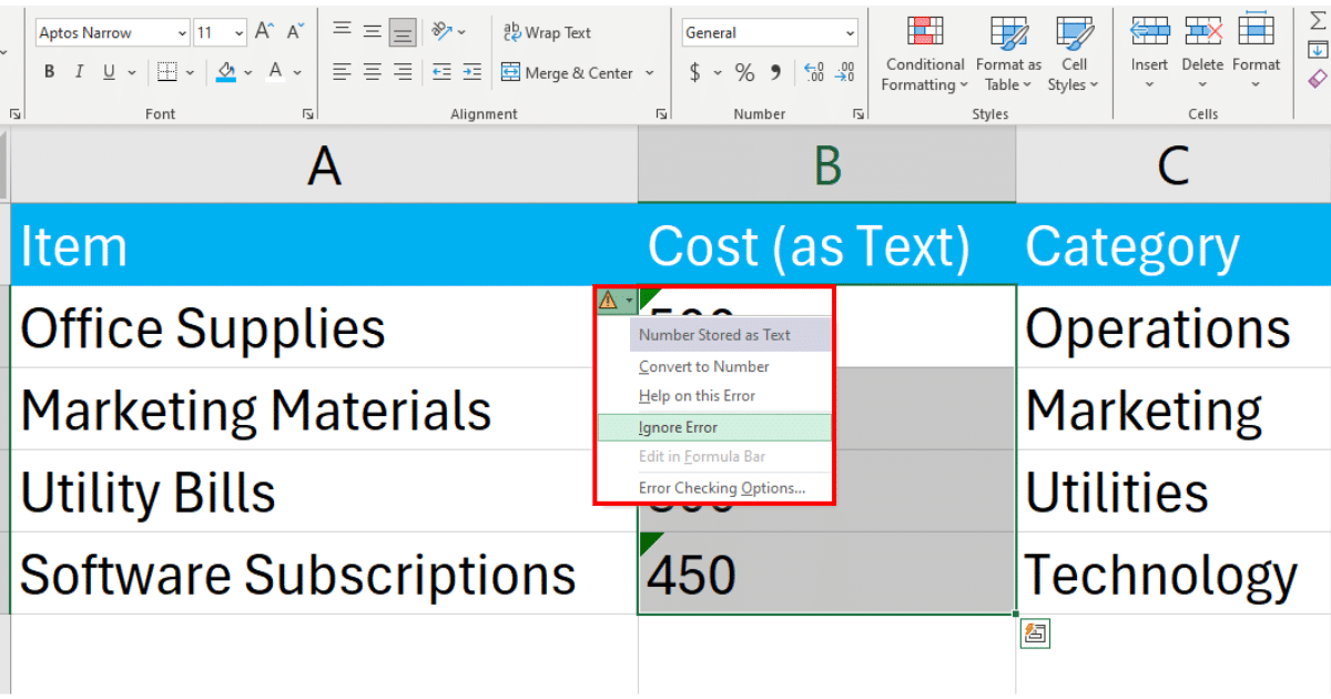
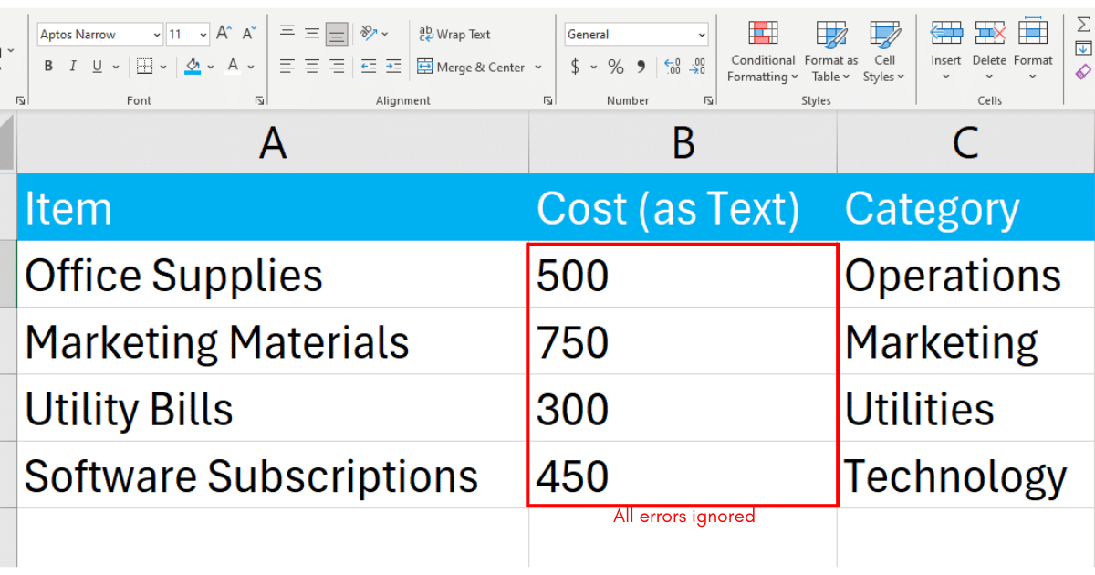
The green triangle will disappear, indicating the error is now ignored.
Method 2: How to Ignore All Errors by Disabling Background Error Checking
Disabling background error checking in Excel allows you to ignore all errors across the entire workbook.
This method is useful when you’re confident about the accuracy of your data and wish to avoid the distraction of these indicators.
Step 1: Open Excel Options
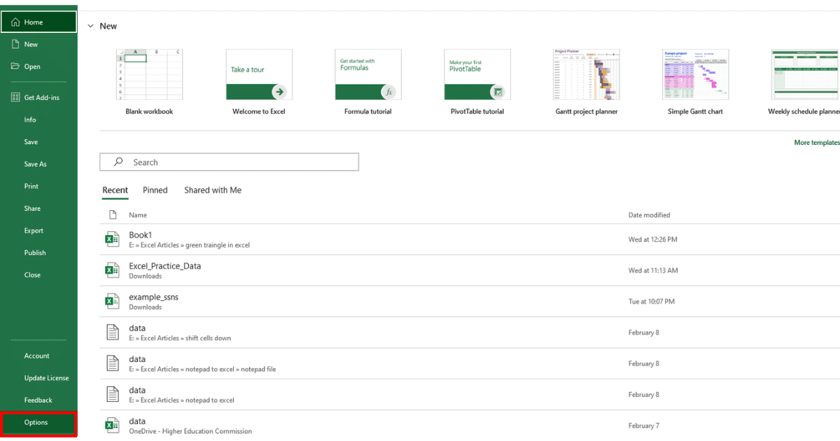
In Excel, click on the File tab in the ribbon.
Select Options from the bottom of the sidebar to open the Excel Options dialog box.
Step 2: Navigate to Formulas Section
In the Excel Options dialog box, click on Formulas in the list on the left side.
Uncheck the box next to Enable background error checking. This action will stop Excel from marking errors with green triangles.
Step 3: Apply And Close
Click OK at the bottom of the Excel Options dialog box to apply your changes and close the dialog.
Excel will ignore all the errors in your worksheet.
Method 3: How to Ignore All Errors by Using the Error Checking Dialog Box
The error-checking dialog box allows you to manage and ignore errors more selectively compared to disabling background error-checking entirely.
Follow the steps below to ignore all errors using this method:
Step 1: Access the Error Checking Dialog
Go to the Formulas tab on the Excel ribbon.
In the Formula Auditing group, click on Error Checking.

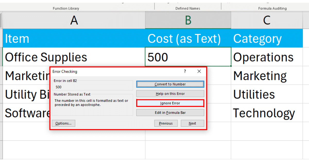
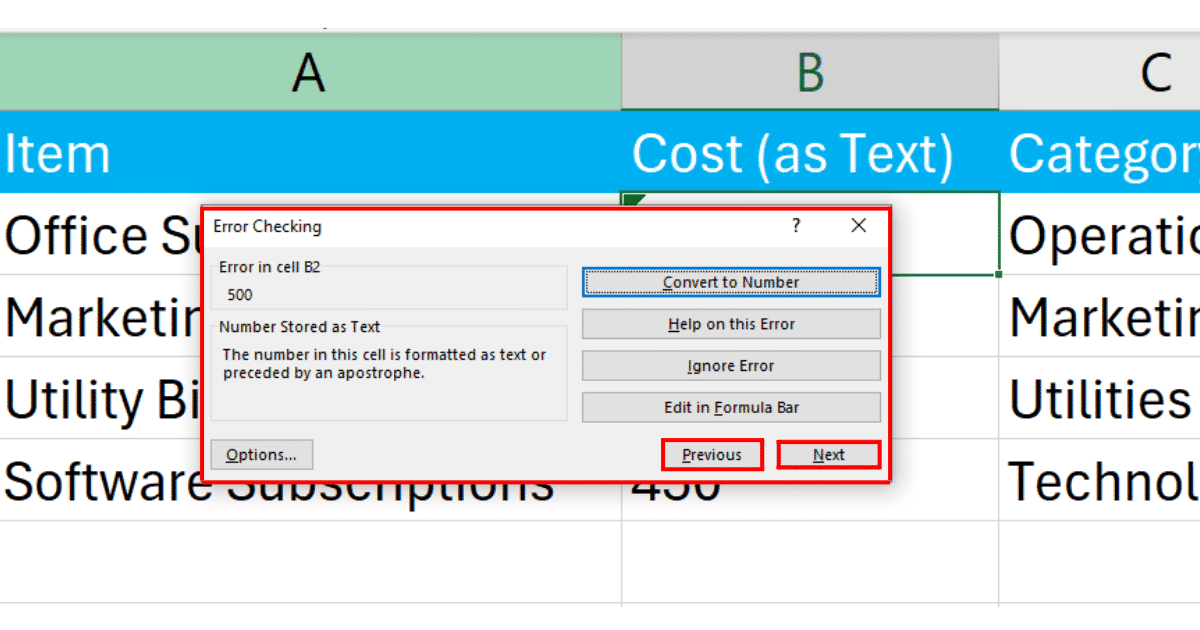
This action opens the Error Checking dialog box, which lists the errors found in the current worksheet.
Step 2: Review Errors
The dialog box will present a list of errors found in your worksheet.
You can navigate through errors using the Previous and Next buttons within the dialog.

Step 3: Ignore Errors
For each error, you have the option to Ignore Error. This will remove the green triangle from the selected error without actually correcting the underlying issue.
You can repeat this for each error listed in the dialog box.

Step 4: Close the Dialog
Once you’ve navigated through all errors and chosen to ignore them or adjusted your settings, click Close to exit the Error Checking dialog box.
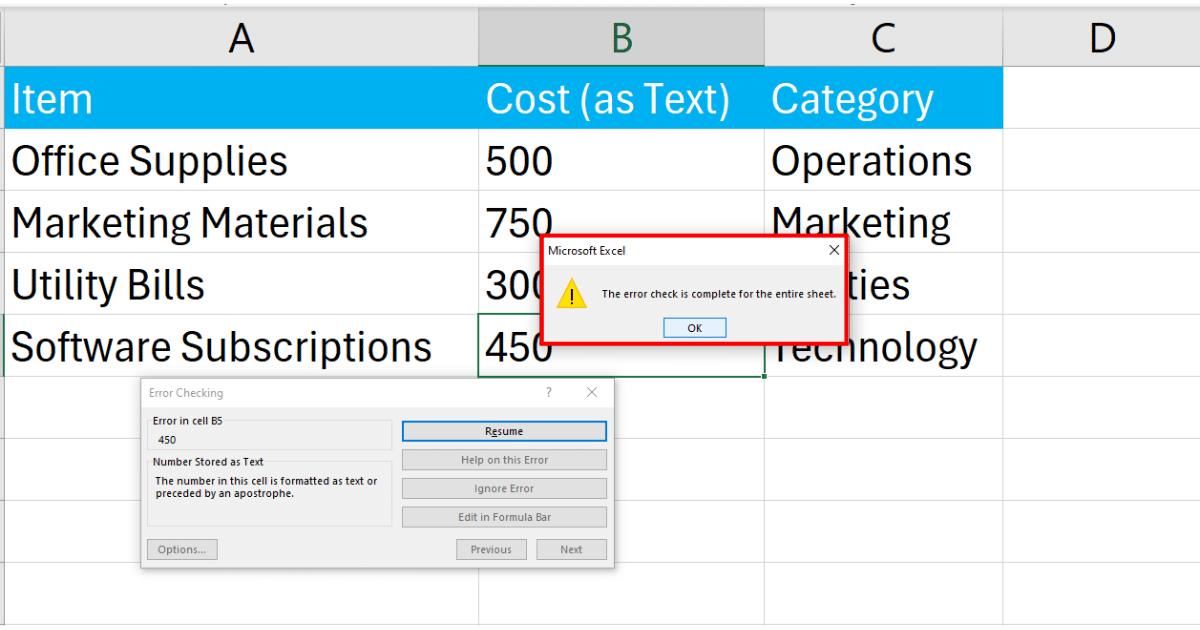
With this method, you can remove all the errors one by one.
Method 4: How to Ignore All Errors Using VBA
You can also ignore all errors in Excel workbook using VBA. It allows for an automated, programmatic approach to dealing with error indicators.
This method is highly efficient, especially when dealing with large datasets or multiple worksheets, as it can apply changes across the entire workbook with a single script execution.
Follow the steps below to ignore all errors using VBA:
Step 1: Open the VBA Editor
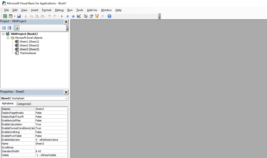
Press Alt + F11 to open the VBA Editor in Excel.
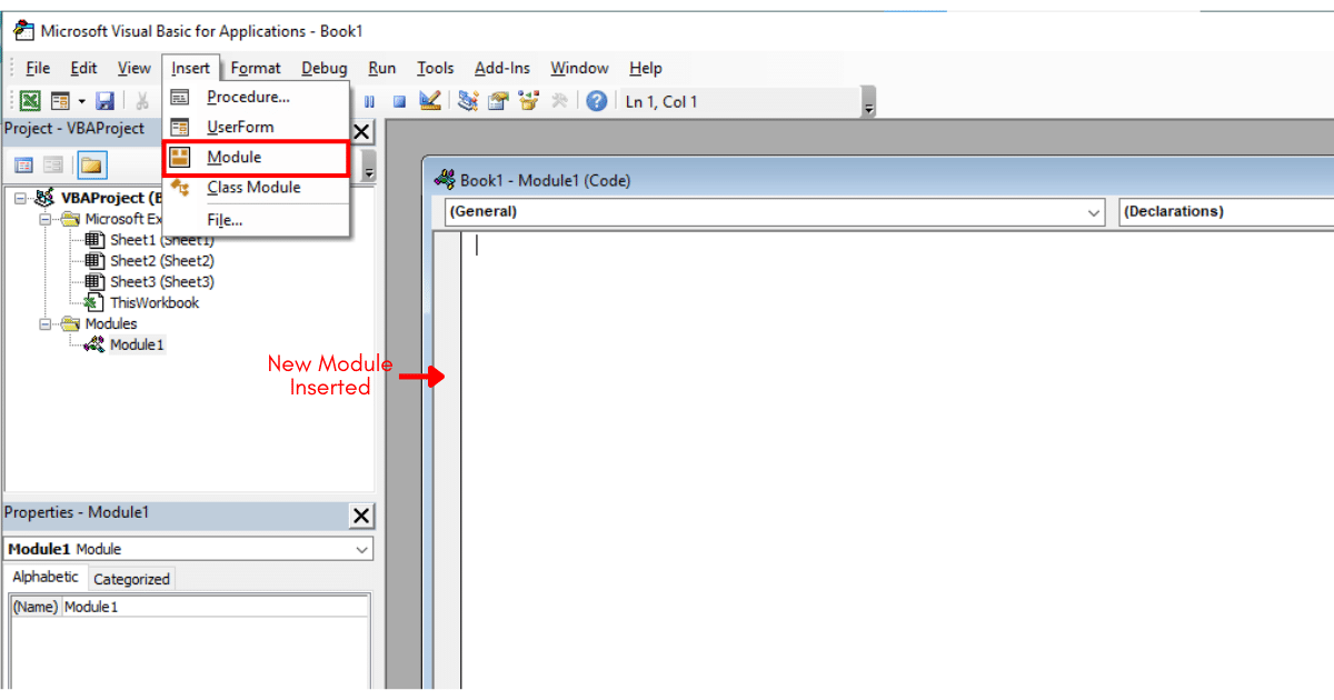
Step 2: Insert a New Module
In the VBA Editor, right-click on any of your workbook’s names in the Project window.
Choose Insert > Module to create a new module.
Step 3: Enter the VBA Code
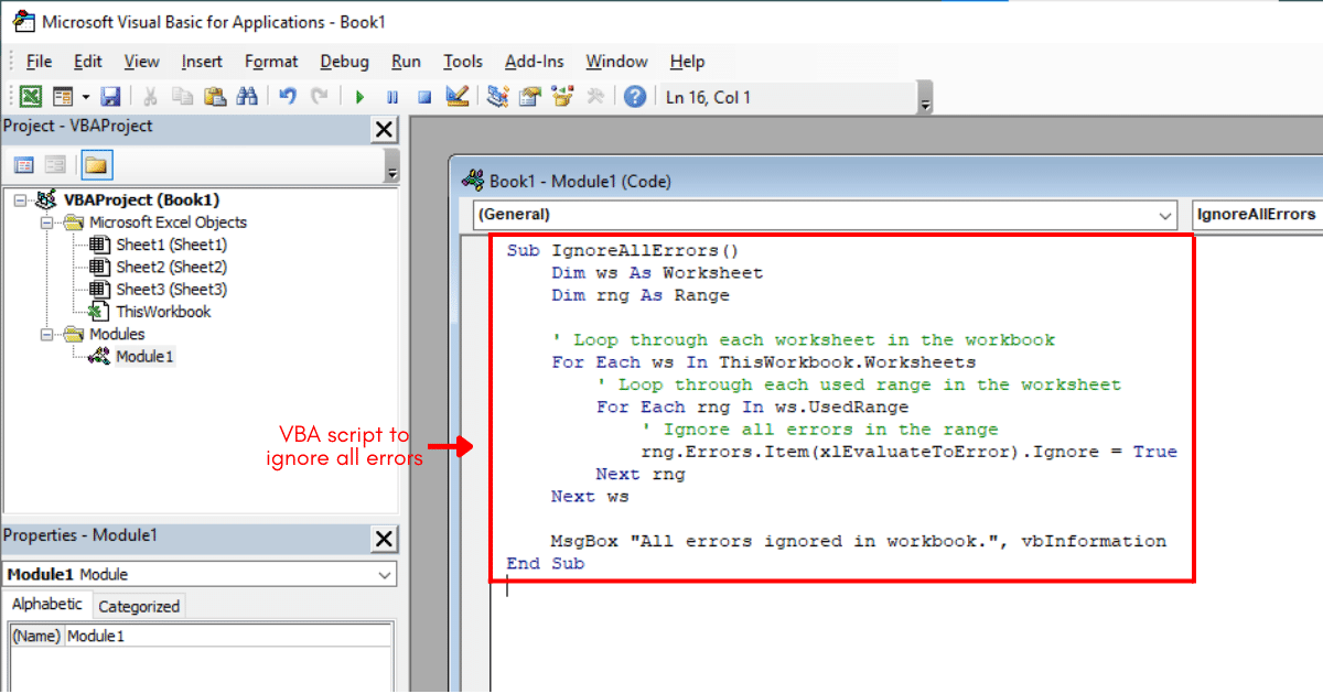
Copy and paste the following VBA script into the module window:
Sub IgnoreAllErrors()
    Dim ws As Worksheet
    Dim rng As Range

    ' Loop through each worksheet in the workbook
    For Each ws In ThisWorkbook.Worksheets
        ' Loop through each used range in the worksheet
        For Each rng In ws.UsedRange
            ' Ignore all errors in the range
            rng.Errors.Item(xlEvaluateToError).Ignore = True
        Next rng
    Next ws

    MsgBox "All errors ignored in workbook.", vbInformation
End Sub
The VBA script IgnoreAllErrors systematically goes through every cell in all worksheets of an Excel workbook and ignores all detected errors, effectively removing the green triangle error indicators from those cells.
Step 4: Run the VBA Script
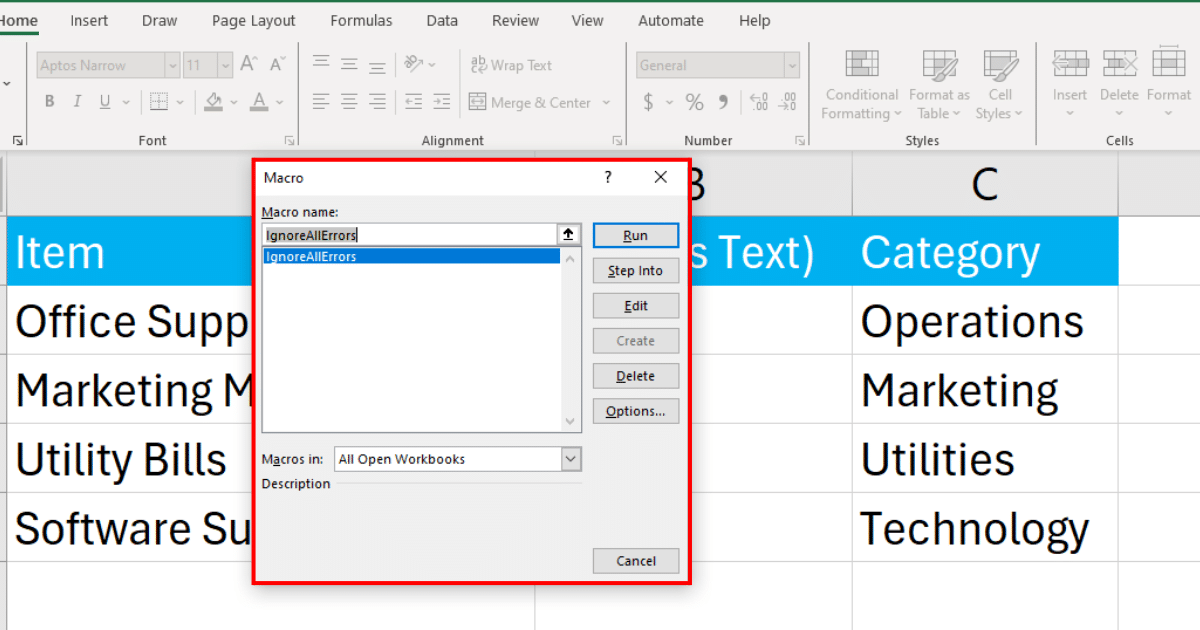
Press Alt + F8 to open the VBA scripts menu.
Select the script you created and then click Run.
Excel will ignore all the errors in your worksheet.
Method 5: How to Ignore All Errors Using IFERROR Function
The IFERROR function allows you to handle common Excel errors directly within formulas.
It allows you to specify an alternative result when a formula would otherwise result in an error, effectively ignoring the error by replacing it with a value or action of your choosing.
Follow the steps below to ignore all errors using the IFERROR Function:
Step 1: Identify the Formula With Error
Determine the formula in your worksheet that might result in an error under certain conditions. You can check the error using multiple error checking options.
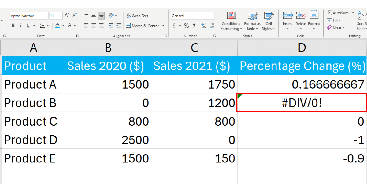
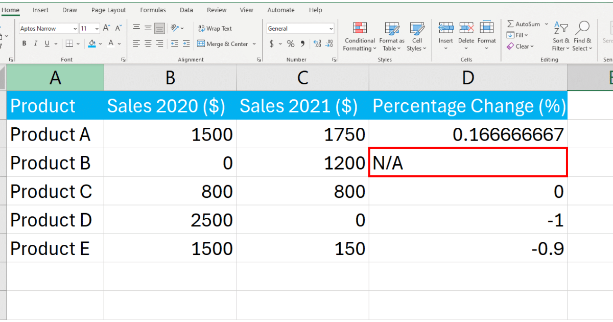
Take a look at the following Excel data:

The highlighted cell has a formula where the error occurs. We must use an IFERROR function to ignore or correct errors in the cell.
Step 2: Apply the IFERROR Function
Wrap the original formula with the IFERROR function. The syntax is as follows:
=IFERROR(value, value_if_error)In the above formula:
value: The original formula or expression you’re evaluating.
value_if_error: The value or action to perform if the original formula results in an error. This could be text like “Error” or “N/A”, a numerical value like 0, or another formula.
In our case, the formula would look like the following:

Step 3: Press Enter
Press Enter and Excel will ignore the error message and replace it with your desired value.
Learn how you can supercharge your analytics journey with EnterpriseDNA by watching the following video:
Final Thoughts
Errors are a natural part of working with data. They signal discrepancies, potential issues, or simple mismatches in our expectations versus reality.
However, not all errors require correction. Sometimes, they arise from data entered in a format Excel doesn’t recognize, or they’re the result of calculations that don’t apply to every scenario.
Recognizing when to fix errors and when to let them be is a skill that enhances your efficiency and clarity in data integrity and management.
Lastly, by mastering the art of ignoring error-checking rules, selectively or globally, allows you to maintain the integrity of your data while presenting it in the most understandable and clean format.
Happy number crunching!
Frequently Asked Questions
In this section, you will find some frequently asked questions you may have when ignoring all errors in Excel.

How can I suppress errors in Excel?
To suppress error messages in Excel, you can use the IFERROR function. This function allows you to replace an error value with custom messages or specific results.
For example, you can use =IFERROR(A1/B1, “Division by zero”) to display a custom message instead of the #DIV/0! error.
How do I ignore error values in Excel formulas?
To ignore error values in Excel formulas, you can use the IFERROR function. Simply wrap your formula in the IFERROR function and specify the desired output if an error is encountered.
For instance, =IFERROR(SUM(A1:A10), 0) will return 0 if there is an error in the SUM function.
What is the function to suppress the divide by zero error in Excel?
To suppress the divide by zero error in Excel, you can use the IFERROR function with the division formula. For example, =IFERROR(A1/B1, 0). This will replace error values with 0.
Alternatively, you can use the IF function combined with the ISERROR function, like this: =IF(ISERROR(A1/B1), 0, A1/B1).
How to turn off Excel errors?
To turn off Excel errors, navigate to File > Options > Formulas, and under Error Checking, uncheck “Enable background error checking.”
This disables Excel’s automatic flagging of errors with green triangles, turning off visual error indicators across your workbook.


