
Rounding allows you to simplify numbers by approximating their values while still retaining a close representation of the original data. There are times when you will want to round values to the nearest thousand.
The most common Excel functions used to round numbers to the nearest thousand are the ROUND, CEILING, and FLOOR functions. Several other functions suit specific scenarios, such as the ROUNDUP or ODD function.
This article shows examples of eight rounding functions and the different results that they produce. You will also learn how to use custom formats to change the display. Finally, you’ll get a taste of using Power Query for this task.

Let’s get started!
What Does Rounding Mean?
In mathematics, rounding to the nearest thousand means approximating a number to the closest multiple of one thousand.
This is done to simplify numbers when the exact value is not necessary, or the focus is on larger trends or patterns.
If you are manually rounding to the nearest thousands, these are the steps:
Identify the digit in the thousands place (the third digit from the right in whole numbers).
Look at the digit immediately to the right of the thousands place digit (the hundreds place digit).
If the hundreds place digit is greater or equal to 5, increase the thousands place digit by 1; otherwise, leave the thousands place digit as it is.
Replace all the digits to the right of the thousands place digit with zeros.
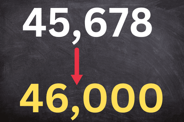
Here are two examples:
rounding 45,678 results in 46,000.
rounding 45,278 results in 45,000.
Alternatives
The method above rounds up or down depending on the value. There are two other common rounding methods:

Rounding up (also known as “ceiling”)
Rounding down (also known as “floor”)
This article shows you how to achieve all these methods in Excel.
Excel’s Rounding Functions
Excel has multiple round functions, allowing for flexibility in your rounding process. Here is a brief overview of them all:
ROUND(number, num_digits)
CEILING(number, significance)
FLOOR(number, significance)
ROUNDUP(number, num_digits)
ROUNDDOWN(number, num_digits)
MROUND(number, multiple)
EVEN – rounding to even-numbered thousands
ODD – rounding to odd-numbered thousands
The functions are available in all modern versions of Excel, including Excel 2016, 2013, 2010, and 2007, as well as Excel for Microsoft 365.
Over the next 8 sections, we’ll take a look at how each function works. Let’s dive in!
1. How to Use the Round Function to the Nearest Thousand in Excel
In Excel, it’s common practice to use the ROUND function to round numbers to the nearest thousand.
The syntax for the ROUND function is:
=ROUND(number, num_digits)
number: The value you want to round to the nearest 1,000
num_digits: The number of decimal places to round to. Use -3 for the nearest thousand.
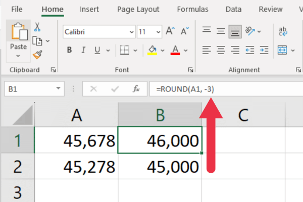
For example, if you want to round the value in cell A1 to the nearest thousand, enter this formula into cell B1:
=ROUND(A1, -3)
This picture shows the function in action:
The function works with both positive and negative values. It also works when the number has a decimal point.
2. How to Use CEILING to Round Up to Nearest Thousand
The CEILING function rounds a given number up to the nearest specified multiple. The syntax is:
=CEILING(number, significance)
number: The number you want to round up.
significance: The multiple to which you want to round the number up.
It can be used to round numbers up to the nearest thousand when you specify a multiple of 1,000.
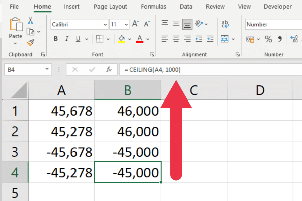
For example, if your value is in cell reference A1, this is the syntax:

=CEILING(A1, 1000)
If the number is 45,278 then the formula will return 46,000.
This function can handle negative numbers and provide consistent results for both positive and negative values. This picture shows the function in action.
3. How to Use FLOOR to Round Down to the Nearest Thousand
The FLOOR function rounds a given number down to the nearest specified multiple. The syntax is:
=FLOOR(number, significance)
number: The number you want to round down.
significance: The multiple to which you want to round the number down.
It can be used to round numbers down to the nearest thousand when you specify a multiple of 1,000.
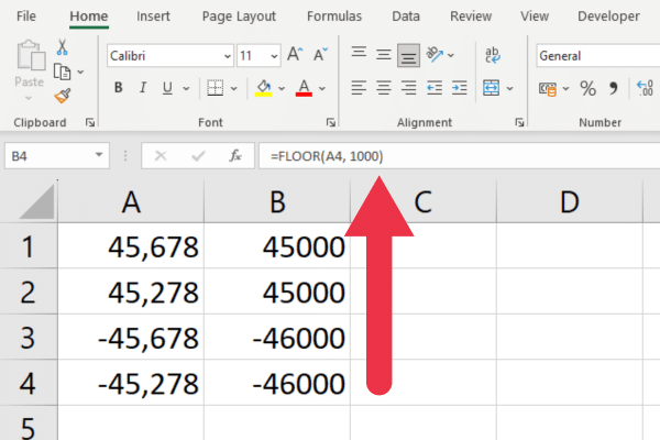
For example, if the number in cell A1 is 45,678 then the formula will return 45,000.
This function will handle negative numbers and provide consistent results for both positive and negative values.
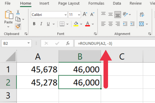
4. How to Round Up to the Nearest Thousand with ROUNDUP
The ROUNDUP function rounds a number up to the specified number of digits. This is the syntax and two arguments:
=ROUNDUP(number, num_digits)
number: the value you want to round.
num_digits: use -3 for the nearest thousand.
For example, if you have the number 45,278, the result will be 46,000.
Note that this is different from the result with the ROUND function, which would automatically round this number down.
This picture shows how different numbers will round up to the same value.
The function works with negative numbers as well.
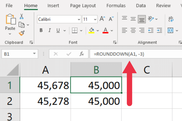
5. How to Round Down to the Nearest Thousand in Excel
The ROUNDDOWN function rounds a number down to the specified number of digits. This is the syntax:
=ROUNDDOWN(number, num_digits)
number: the value you want to round.
num_digits: use -3 for the nearest thousand.
For example, if you have the number 45,678, the result will be 45,000.
Note that this is different from the result with the ROUND function, which would automatically round the number up.
This picture shows how two different numbers will round down to the same value.
This function works with negative numbers as well.

6. How to Use the MROUND Function
The MROUND function is similar to ROUND but has a different syntax:
=MROUND(number, multiple)
The first argument is the same. However, the second argument specifies the nearest multiple.
For example, if you want a number rounded to the nearest ten, you would supply a 10 in this parameter. Similarly, to round up to the nearest one thousand, you supply 1,000 like this:
=MROUND(number, 1000)
For example, if you have the number 45,678, the result will be 46,000.
Note that this function does not work with negative numbers. This picture shows it in action with positive and negative numbers.
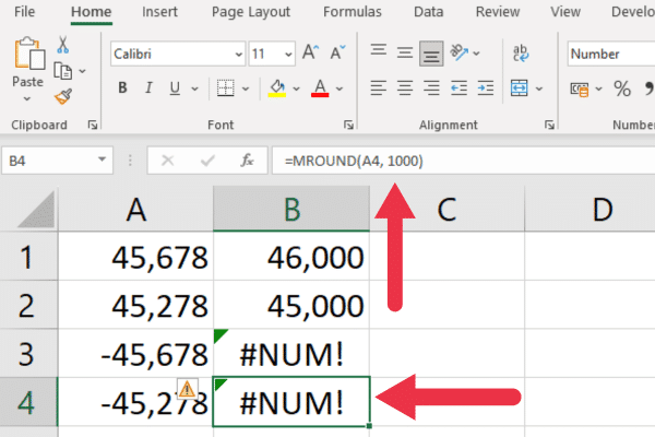
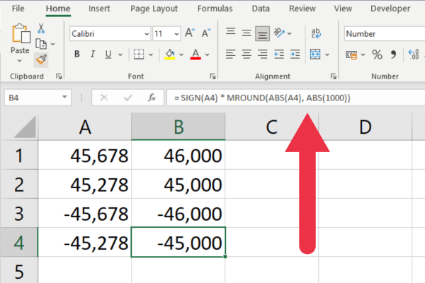
How to Avoid Errors with Negative Numbers
To avoid #NUM! errors with negative numbers, follow these steps:
Wrap the number and the multiple in the ABS (absolute value) function.
Apply the original sign back to the result using the SIGN function.
This modified formula works when operating on cell A1:
= SIGN(A1) * MROUND(ABS(A1), ABS(1000))
This picture shows the errors eliminated with the above formula:
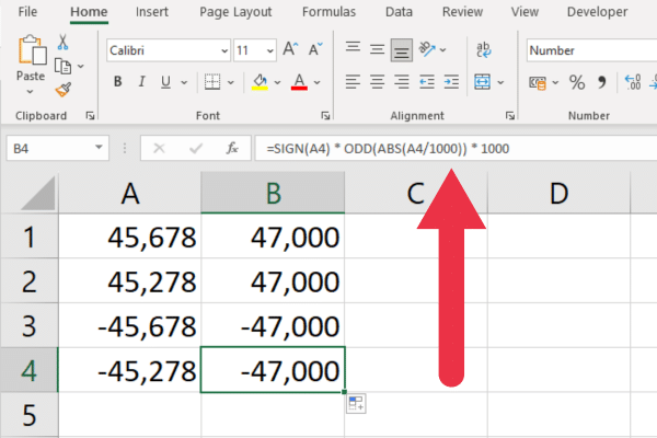
7. How to Use the Odd Function
The ODD function in Excel rounds a positive number up to the nearest odd number and a negative number down to the nearest odd number.
To round a number in cell A1 to the nearest odd thousand, you can use the following formula:
=SIGN(A1) ODD(ABS(A1/1000)) 1000
Replace A1 with the cell containing the number you want to round.
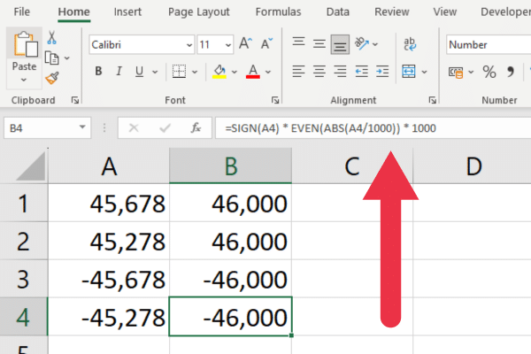
8. How to Use the EVEN Function
The EVEN function in Excel rounds a positive number up to the nearest even number and a negative number down to the nearest even number.
To round a number in cell A1 to the nearest odd thousand, you can use the following formula:
=SIGN(A1) EVEN(ABS(A1/1000)) 1000
Replace A1 with the cell containing the number you want to round.
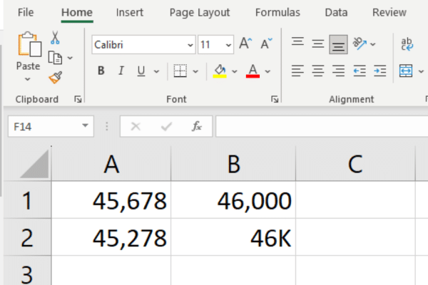
How to Use a Custom Number Format
You can use a custom number format to display cell values in thousands while retaining the original underlying value for calculations.
In other words, the cell value itself doesn’t change because you simply change how it’s displayed. Any calculations use the underlying value.
To set a custom format, follow these steps:
Select the cell or range of cells containing the numbers you want to format.
Right-click the selected cell(s) and select “Format Cells” to open the number tab.
In the Category box select Custom as the option.
Enter the custom format you want to apply. There are some suggestions below for different formats.
Click “OK”.
There are several formats for displaying thousands. Here are two alternatives to enter into the custom type box:
#0,”,000″
#0,”K”
The first of these formats replaces the last three digits with “000”. The second replaces the last three digits with “K”, a common symbol for one thousand. Both suppress the decimal place.
The picture below shows the unformatted original number in one column and the custom format in the other column. The result of the first format in cell B1 and the second format in cell B2.
This kind of formatting is useful for printouts of your data. You can have both unformatted and formatted columns in the spreadsheet, while only choosing the latter when you set your print area.
One issue that users may experience with custom formats is that the calculations may appear to be “wrong”. You may want to add an explanatory comment to a table or chart to decrease confusion.
Rounding with Power Query
This article has focused on in-built Excel functions for rounding. You can also use the functions provided by the M language in the Power Query editor.
Some of the common rounding functions in Power Query are:
Number.Round
Number.RoundUp
Number.RoundDown
For example, if you want to round the values in a column named “Amount” to the nearest integer, you would use the following formula in the “Custom Column” window:
= Number.Round([Amount], 0)
Rounding functions are often used to tidy up messy numeric data. Power Query lets you clean up both numbers and text at the same time. Check out this video to see this in action:
Final Thoughts
So, there you have it! Rounding numbers to the nearest thousand in Excel isn’t so hard after all. Whether you’re using the ROUND, MROUND, or FLOOR and CEILING functions, you can now confidently manipulate your data to suit your specific needs.
Mastering these rounding functions in Excel not only enhances your spreadsheet skills but also enables you to deliver more accurate and professional-looking reports.
Remember, Excel is all about making your life easier, and these functions are just a few examples of its data-crunching prowess. So, don’t shy away from diving in and getting to grips with Excel’s array of functions — you never know when they’ll come in handy.
Keep exploring, keep learning, and you’ll find that Excel is full of surprises and time-saving tricks! Happy rounding!


