
Some tasks in Excel involve comparing values to see if they are equal to or greater than a specific criterion. This is where the greater than or equal to function, a type of logical operation, comes in handy.
With Excel’s greater than or equal function, you can evaluate conditions to return TRUE or FALSE results.
This function is represented by the “>=” symbol and can be used in formulas, conditional formatting rules, or logical tests.

The greater than or equal to comparison operator (>=) returns TRUE if the first value is greater than or equal to the second value.
In this article, you’ll learn how to implement the greater than or equal to feature in Excel.
Let’s get started!
Introducing Excel’s Comparison Operators

Excel’s comparison operators, including the greater-than-or-equal-to operator (>=), are integral to performing logical operations and conditionally formatting your data.
1. Comparison Operators for Numbers
| Operator | Description | Example | Result Description |
|---|---|---|---|
> | Greater Than | A1 > B1 | TRUE if A1 exceeds B1 |
>= | Greater Than or Equal to | A1 >= B1 | TRUE if A1 is greater than or equal to B1 |
< | Less Than | A1 < B1 | TRUE if A1 is less than B1 |
<= | Less Than or Equal to | A1 <= B1 | TRUE if A1 is less than or equal to B1 |
= | Equal to | A1 = B1 | TRUE if A1 is equal to B1 |
<> | Not Equal to | A1 <> B1 | TRUE if A1 is not equal to B1 |
To compare numeric values, use these comparison operators:
- Greater Than: Return TRUE when the first number exceeds the second, e.g., A1 > B1.
- Greater Than or Equal to: Return TRUE when the first number is greater than or equal to the second, e.g., A1 >= B1.
- Less Than: Return TRUE when the first number is less than the second, e.g., A1 < B1.
- Less Than or Equal to: Return TRUE when the first number is either less than or equal to the second, e.g., A1 <= B1.
- Equal to: Return TRUE when the first number is equal to the second, e.g., A1 = B1.
- Not Equal to: Return TRUE when the first number is not equal to the second, e.g., A1 <> B1.
2. Comparison Operators with Text
| Operator | Description | Example | Result Description |
|---|---|---|---|
= | Equal to | "apple" = "apple" | TRUE if both text values are identical (case-insensitive) |
<> | Not Equal to | "apple" <> "oranges" | TRUE if text values are different (case-insensitive) |
Excel also supports comparison operators when dealing with text values. The rules for text comparison are as follows:

- Text operators can only check equality (i.e., = and <>).
- The comparison is case-insensitive, so “a” and “A” are considered the same.
- If a cell contains a non-text value (a number, date, Boolean, or error), Excel treats it as an empty string for the purpose of comparison.
- The = operator evaluates to TRUE if the two compared values are identical and FALSE if not. This means that “apple = apple” evaluates to TRUE, while “apple = oranges” evaluates to FALSE.
All the comparison operators evaluate to a logical value, such as TRUE or FALSE. This is because they are used in logical tests to compare one or more values.
Now, let’s explore the basic functionality of the greater than or equal to the operator in Excel.
The Basics of Greater Than or Equal to

1. Referencing Cell Values
To compare cell values in Excel, you can use the greater than or equal to the operator (>=). To follow the syntax, simply use the following formula in an empty cell:
Assume that Cell A1 has a value of 9 and Cell B1 has a value of 6. The formula will return TRUE, since the value in Cell A1 (9) is greater than in Cell B1 (6).
If the values are equal, the formula will also return TRUE. For example, if both A1 and B1 have a value of 7, the formula will return TRUE.
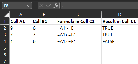
If Cell A1 has a value of 4 and Cell B1 has a value of 6, the formula will return FALSE.
You can also use named ranges in your formulas, making them more readable and easier to maintain.
=Sales1 >= C1Simply replace the cell references with the named range. For example, if you have a named range “Sales” that refers to cells A1:B10, you can rewrite the formula as follows:
Next, we’ll delve into using constants in comparison formulas.
2. Working with Constants
You can also compare a cell value with a constant. In this case, you specify the constant value directly in the formula instead of referring to another cell.
For example, the following formula compares the value in Cell A1 with the constant value 5:
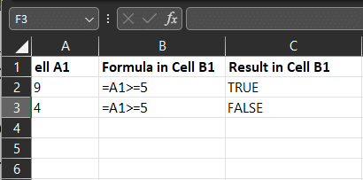
The formula will return TRUE if the value in Cell A1 is greater than or equal to 5, and FALSE otherwise. If A1 is 9, the result is TRUE. If A1 is 4, the result is FALSE.
Remember that the greater than or equal to the operator (>=) is a comparison operator and can only be used to check if a value is greater than or equal to another.
You cannot use it to directly change the value in a cell. For instance, the following formula is not valid and will return an error:
While you cannot directly change the value of a cell with the greater than or equal to operator (>=), you can use it in conjunction with other functions to perform conditional operations in Excel.

Next up, let’s take a deeper look at conditional formulas.
Understanding Conditional Formulas

In Excel, conditional formulas are used to apply specific calculations or actions based on a set of criteria or conditions.
They consist of a logical test followed by a value or expression to be evaluated when the test is TRUE, and, optionally, a different value or expression when the test is FALSE.
1. Basic Syntax of Conditional Formulas
| Condition | Value if True | Value if False |
|---|---|---|
| TRUE | “Pass” | “Fail” |
| FALSE | “Accepted” | “Rejected” |
Excel supports several conditional formulas, such as the IF, SWITCH, and IFS functions. Each of these functions follows a basic syntax, as shown below:
\\[condition\]\ is a logical test or expression that evaluates to TRUE or FALSE.
\\[value\_if\_true\]\ is the value or expression to be returned if the condition is TRUE.
\\[value\_if\_false\]\ is the value or expression to be returned if the condition is FALSE (optional for the IFS function).
Moving on, let’s understand the essentials of conditional formulas in Excel.
2. IF: A Basic Conditional Formula
| Value to Check | Formula | Result |
|---|---|---|
| 8 | =IF(A2>=10, "Yes", "No") | “No” |
| 12 | =IF(A3>=10, "Yes", "No") | “Yes” |
IF is the most commonly used conditional formula in Excel. It allows you to check a condition and return one value if it is TRUE or a different value if it is FALSE.
The syntax for the IF function is as follows:
- Logical\_test – This is the condition you want to check. It can be a value, a cell reference, or an expression.
- Value\_if\_true – This is the value or expression to return if the condition is TRUE.
- Value\_if\_false – This is the value or expression to return if the condition is FALSE.
Now, let’s examine the IF function and its usage with the greater than or equal to operator.
3. IF, Greater Than Or Equal To Example
| Cell A1 | Formula in Cell B1 | Result in Cell B1 |
|---|---|---|
| 15 | =IF(A2>=10, "Yes", "No") | “Yes” |
| 9 | =IF(A3>=10, "Yes", "No") | “No” |
Let’s take an example of a simple IF statement to understand the basics. The following IF function compares the value in cell A1 with 10. If the value is greater than or equal to 10, it returns “Yes”; otherwise, it returns “No”:
The function checks whether the value in cell A1 is greater than or equal to 10. If it is, it returns “Yes”. If it is not, it returns “No”.
Next, we dive into additional functions that enhance Excel’s functionality for logical operations.
4. Additional Functions for Enhanced Functionality
Excel also contains other conditional functions, such as IFS and SWITCH, that can perform more complex logical tests with multiple conditions.
| Score | Formula | Grade |
|---|---|---|
| 92 | =IFS(A2>=90, "A", A2>=80, "B", A2>=70, "C") | “A” |
| 85 | =IFS(A3>=90, "A", A3>=80, "B", A3>=70, "C") | “B” |
| 75 | =IFS(A4>=90, "A", A4>=80, "B", A4>=70, "C") | “C” |
- The IFS function allows you to check multiple conditions and return a value corresponding to the first TRUE condition. The syntax is as follows:
| Category Number | Formula | Category Name |
|---|---|---|
| 1 | =SWITCH(B2, 1, "Books", 2, "Electronics", "N/A") | “Books” |
| 2 | =SWITCH(B3, 1, "Books", 2, "Electronics", "N/A") | “Electronics” |
| 3 | =SWITCH(B4, 1, "Books", 2, "Electronics", "N/A") | “N/A” |
The SWITCH function is similar to IFS but more concise and accessible to read when dealing with multiple conditions.
Moving on, let’s discuss the nuances of case-sensitive and case-insensitive comparisons in Excel.
5. Case-Sensitive and Case-Insensitive Comparisons
| Comparison Type | Description | Example | Result Description |
|---|---|---|---|
| Case-Insensitive | Excel’s default behavior for text comparisons | "apple" = "Apple" | TRUE, as Excel ignores case differences |
| Case-Sensitive | Requires special functions like EXACT | EXACT("apple", "Apple") | FALSE, as Excel treats different cases as distinct |
By default, Excel performs case-insensitive comparisons in conditional formulas. This means that “apple” and “Apple” will be considered the same in logical tests. There is no need to use case-insensitive operators like LOWER or UPPER.
Now, we’ll explore how to apply conditional formulas within Excel tables.
6. Apply Conditional Formulas in Excel Tables
| Temperature | Formula | Status |
|---|---|---|
| 101 | =IFS(A2>99, "Fever", A2>=97, "Normal", "Hypothermia") | “Fever” |
| 98.6 | =IFS(A3>99, "Fever", A3>=97, "Normal", "Hypothermia") | “Normal” |
| 95 | =IFS(A4>99, "Fever", A4>=97, "Normal", "Hypothermia") | “Hypothermia |
IF formulas can only have a single logical\_test and a single value\_if\_true and value\_if\_false. However, you can use the IFS function to test multiple conditions in a single formula.

Next, let’s delve into conditional formatting using the greater than or equal to operator.
Conditional Formatting with the Greater Than or Equal To Operator

In Excel, conditional formatting is a feature that allows you to format cells that meet specific criteria automatically. Conditional formatting can help you visually highlight important information in your data, such as values greater than or equal to a given threshold.
1. Accessing the Conditional Formatting Tool
To access the conditional formatting tool in Excel, follow the steps below:
- Select the cells that you want to apply the conditional formatting to.
- Go to the “Home” tab on the Excel ribbon.
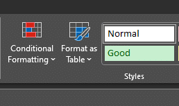
- Click on the “Conditional Formatting” button in the “Styles” group
This will open the conditional formatting menu, where you can choose from predefined conditional formatting rules or create your own custom rule.
Moving on, let’s look at how to create a new conditional formatting rule.
2. Creating a New Conditional Formatting Rule
To create a new conditional formatting rule in Excel, follow these steps:
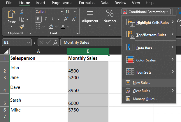
- Select the cells you want to apply the formatting to.
- Click on “Conditional Formatting” > “New Rule.”
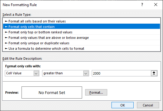
- Choose “Format only cells that contain” under the “Select a Rule Type” section.
- In the “Format only cells with” section, select “Cell Value” from the first drop-down list, “greater than or equal to” from the second drop-down list, and enter the desired value in the third text box.
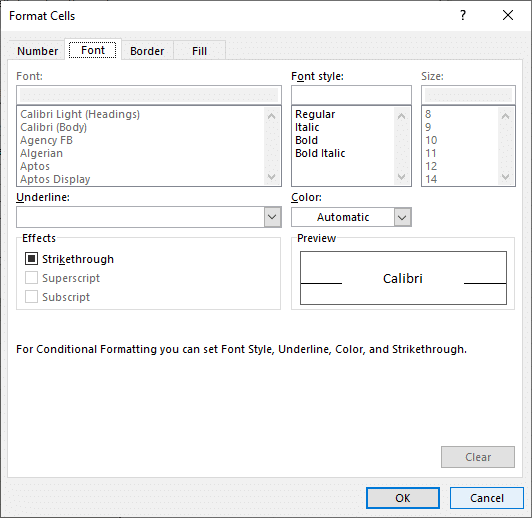
- Click the “Format” button, choose the desired formatting options (e.g., font color, fill color, or borders), and click “OK” to apply the formatting.
- Click “OK” in the “New Formatting Rule” dialog box to confirm the rule.
The selected cells will now be formatted according to the conditional formatting rule, highlighting cells containing values greater than or equal to the specified threshold.
Moving on, we’ll wrap up with final thoughts on using the greater than or equal to operator in Excel.
Final Thoughts

Excel is a powerful tool with various functions designed to make your data analysis process more efficient and accurate.
The greater than or equal to operator (>=) is a key tool that enables you to compare numerical values and make informed decisions based on your analysis.
In this guide, you have learned:
- The syntax and usage of the greater than or equal to the operator (>=) in Excel.
- How to use the operator in simple number comparison formulas and more complex tasks like conditional formatting and logic flow in the IF statement.
- Maintaining consistency in referencing cell values, case-sensitive comparisons, and IF statement arguments is important.
- How to create and apply conditional formatting rules using the greater than or equal to operator (>=) to highlight specific data points in your charts.
By mastering the techniques discussed in this article, you can work with your data more effectively, confidently apply the greater than or equal to the operator in your analysis, and make better-informed decisions based on a thorough understanding of your data.
Do you want to learn more about interesting subjects like Developing data models in the real world?
Frequently Asked Questions
How do I apply greater than and equal to conditions in Excel?
To apply the greater than or equal to condition in Excel, you can use the logical operators “>=” in a formula. For example, the formula “=A1 >= 10” will return TRUE if the value in cell A1 is greater than or equal to 10, and FALSE otherwise.
How to use the AND function with greater than or equal to?
When using the AND function in combination with the greater than or equal to operators, you can evaluate multiple criteria within a single formula.
For instance, the formula “=AND(A1 >= 10, B1 >= 20)” will return TRUE only if the values in cells A1 and B1 are greater than or equal to 10 and 20, respectively.
What is the difference between the greater than and greater than or equal to Excel operators?
The greater than operator (>) returns TRUE if the first value is strictly greater than the second value. On the other hand, the greater than or equal to operator (>=) returns TRUE if the first value is either greater than or equal to the second value.
In other words, for the second operator, it considers the values to be equal as well, returning a TRUE in that case.
How do I highlight cells based on a condition, such as greater than or equal to?
Using conditional formatting, you can highlight cells in Excel based on a condition like greater than or equal to. To do this, select the cells you want to apply the formatting to, go to the “Home” tab, click “Conditional Formatting,” and choose “New Rule.”
Then, select “Format only cells that contain,” choose “Cell Value” in the first dropdown and “greater than or equal to” in the second dropdown. Finally, enter the value you want to compare the cells with and define the formatting to be applied when the condition is met.
How to Use the Greater Than or Equal To Operator in Excel?
To use the greater than or equal to operator (>=) in Excel, simply type the operator between two values or cell references in a formula. For example, =A1 >= B1 will return TRUE if the value in cell A1 is greater than or equal to the value in cell B1.
Can I Use Greater Than or Equal To in Conditional Formatting?
Yes, you can use the greater than or equal to operator in conditional formatting. To do this, create a new rule in the conditional formatting options, select ‘Format only cells that contain’, and then choose ‘Cell Value’ and ‘greater than or equal to’ from the dropdown menus.
Enter the value you want to compare against, and set the desired formatting.


