In this tutorial, I’ll discuss how to use the Well Known Text feature in the Power BI icon map visual. This blog post will further explain the use of Power BI in geospatial projects.
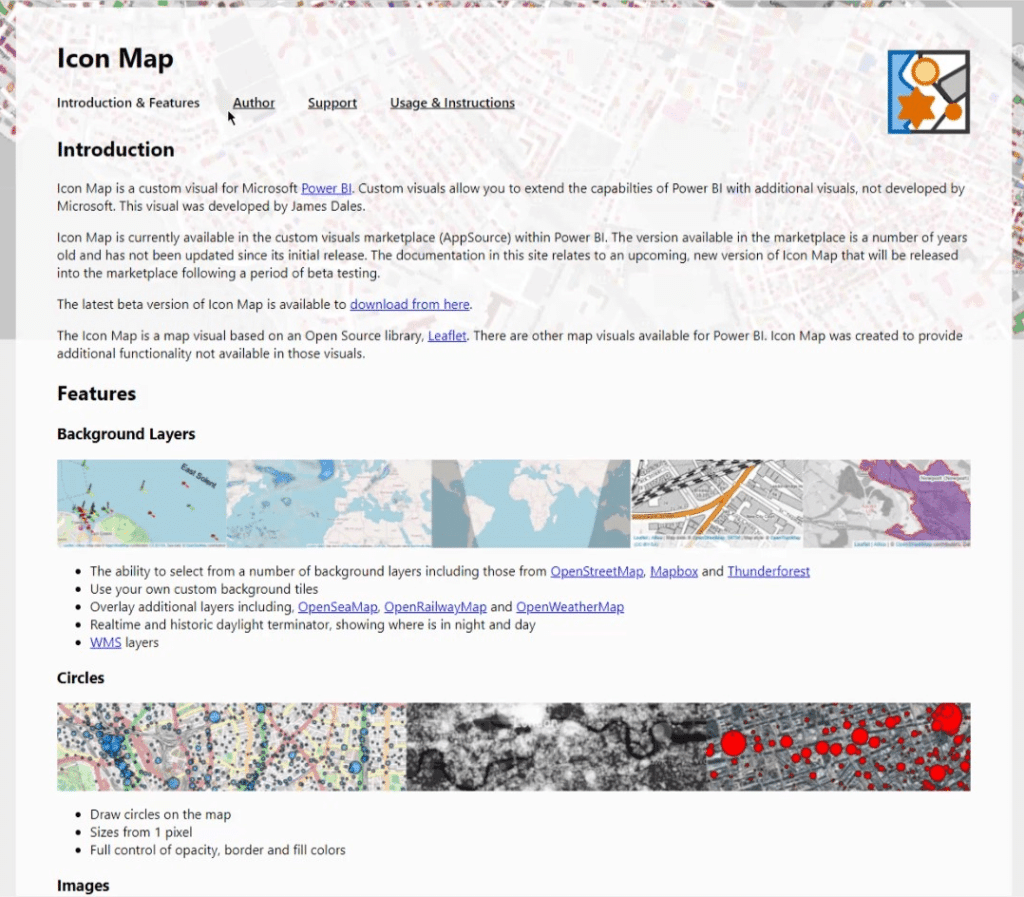
The Power BI Icon Map is one of the most versatile and complex mapping visuals. It offers functionality that other map visuals still lack. It supports various map formats, tooltips, and claims better data security.
For visualizing and analyzing flows such as delivery routes or gas lines, the Icon Map visual offers considerable advantages.

This tutorial is not a demonstration of all the things that the Icon Map can do. This is merely focused on the context of using Well Known Text (WKT) strings.
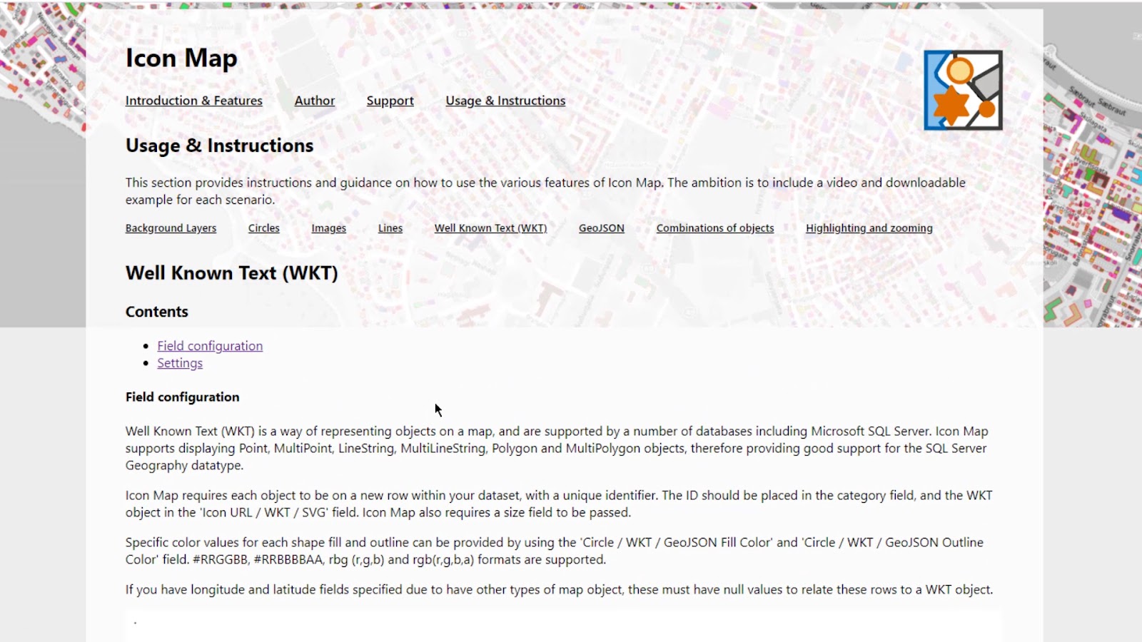
Well Known Text (WKT) In Power BI Icon Map
Well Known Text strings are combinations of longitude and latitude separated by a dot. Combining these in one record creates lines, shapes, or polygons.
You can easily convert your latitude and longitude data in Power Query if you don’t have a Well Known Text string.
You can import the Power BI Icon Map visual from this website (as of this writing, this is still in beta version).
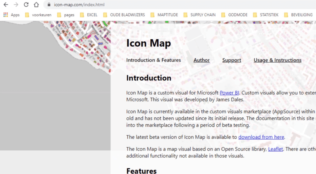
There are lots of working examples on this webpage. However, the visual and the app source do not support all recent changes. According to James Dales (the developer), approval from Microsoft for the beta version is pending as of this writing.
Sample Scenario For Using WKT Strings In Power BI Icon Map
For the first example, I’ll be showing how to display multiple layers with WKT strings for gas lines. I downloaded some information from a website of a gas provider in the Netherlands. I’ve taken the stations and the pipelines just to create this example.

1. Merging Queries
The first part of this example is for merging queries.
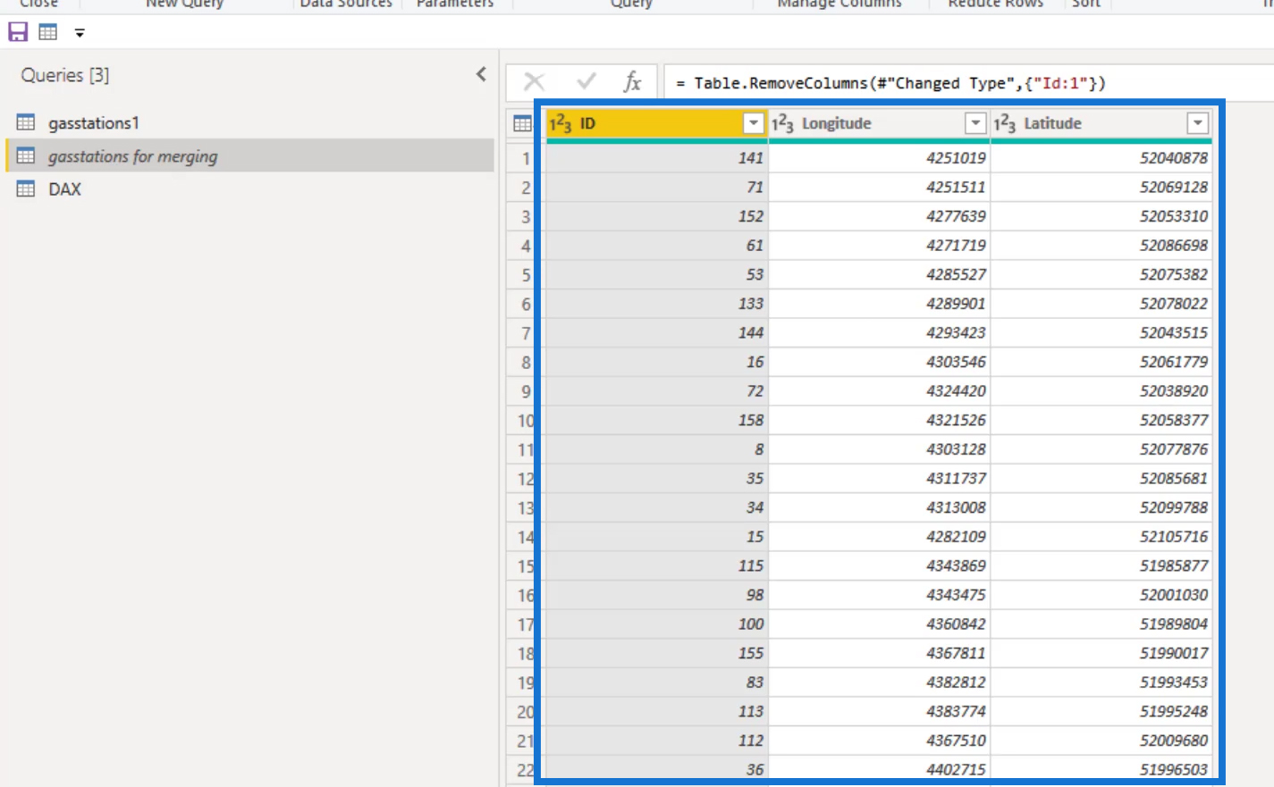
The “gasstations for merging” query contains the ID, Longitude, and Latitude columns.
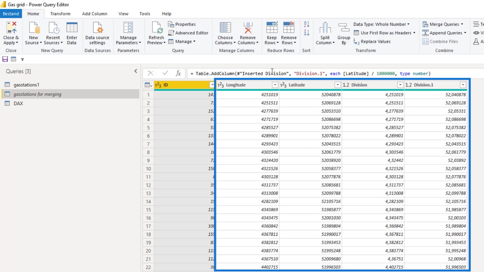
First, I created the longitude and latitude in the 2 division columns by reworking the numbers from the Longitude and Latitude columns. As you can see, the Longitude is similar to the Division column and the Latitude is similar to the Division.1 column.
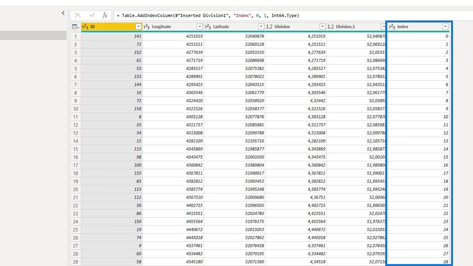
Then, I added the Index column.
I removed the Longitude and Latitude columns.
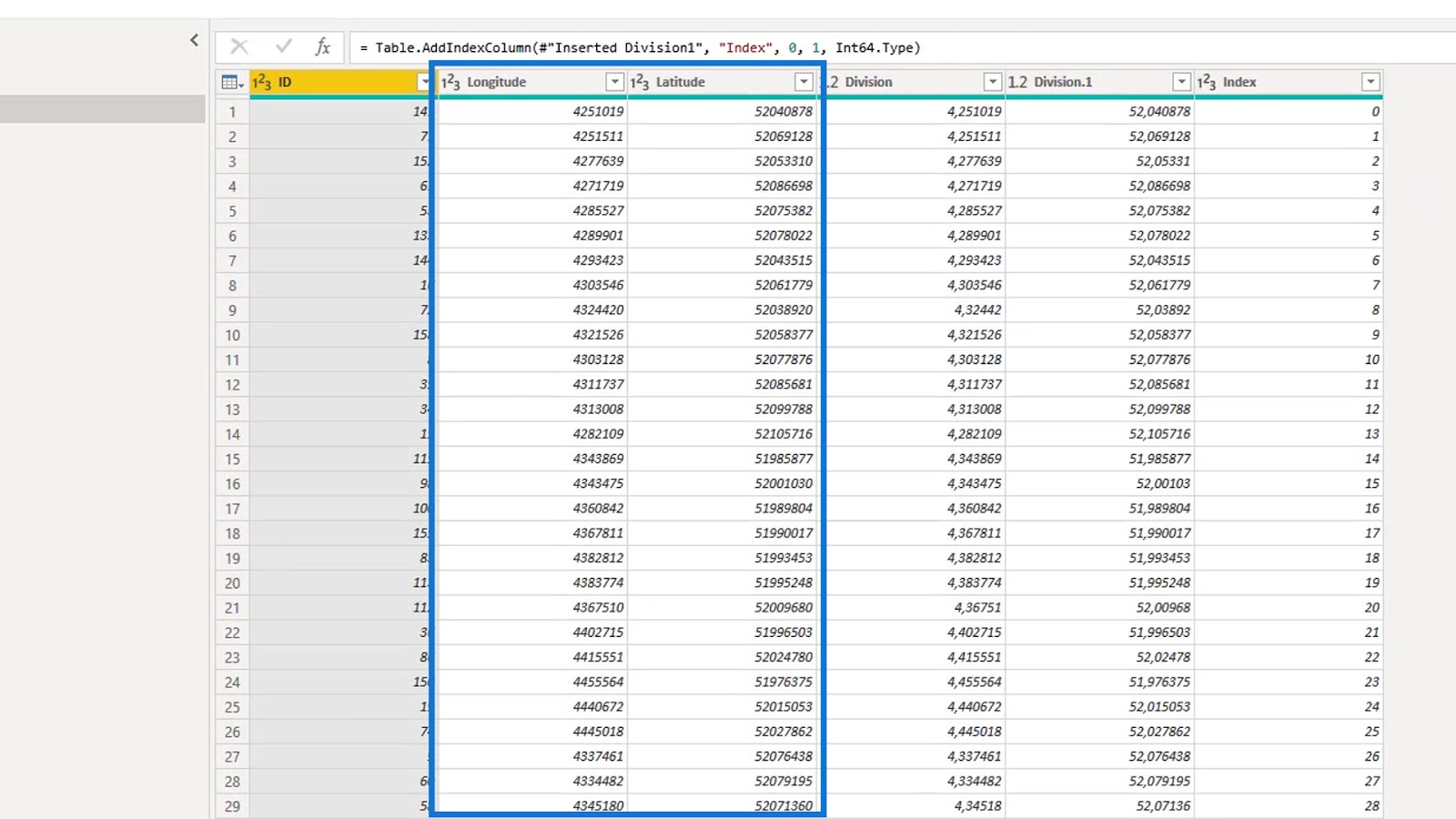
After that, I rounded the reworked latitude and longitude to five digits.
Rounding them to five digits results in an accuracy of about one meter, which is good enough in this scenario. Normally, I round down to four just to save more memory.

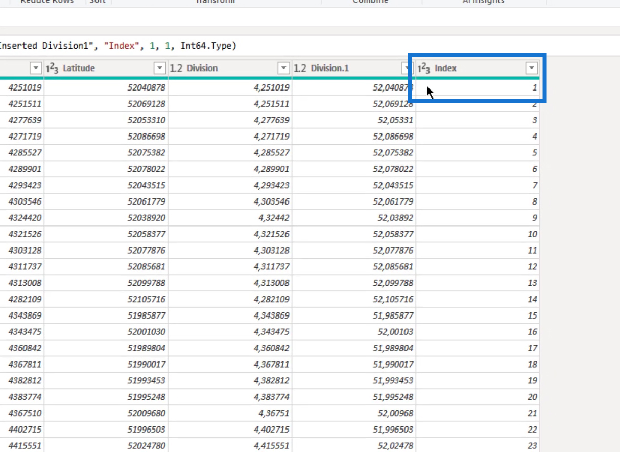
I duplicated the “gasstations for merging” query which has a zero-based index column and named it as “gasstations1” query.
In this query, I created another Index column that starts with 1.
My goal in this query is to create pairs of longitude and latitude for each gas station. Then, combine two sequential pairs into one text string in one record. This will represent a section of the pipeline between stations.
I used the Index column to merge the two queries. As a result, the record with 1 as its index in the “gasstations1” query and the record with 1 as its index in the original query (gasstations for merging) will be merged.
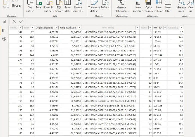
I followed the sequence in the ID column and connected the stations into two pairs.
So, 141 and 71 are adjacent stations as shown in one record. As a pair, they represent that particular section of the gas line. That also goes for 71 and 152, and the succeeding records in the ID column.

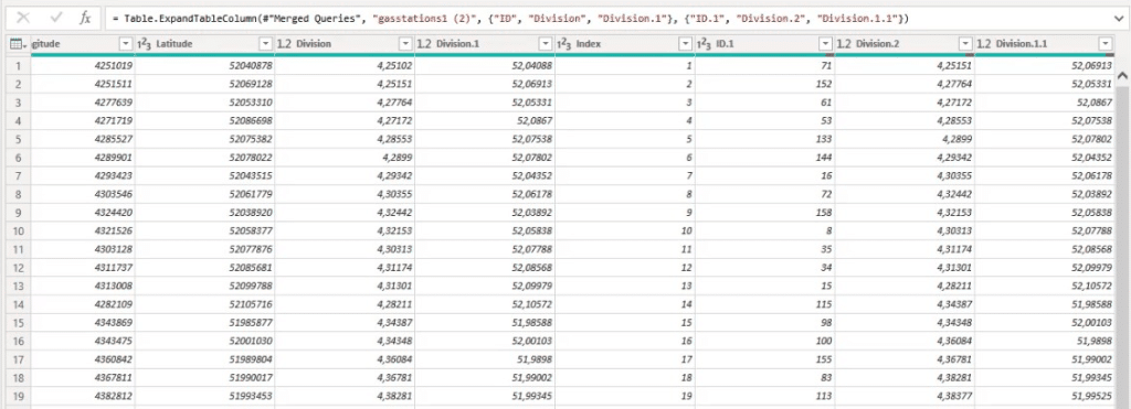
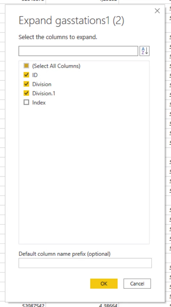
2. Expanding The Table
After merging the queries based on the Index column, I need to expand the table and keep the ID, Latitude, and Longitude columns. The ID is used as the two station part of the Well Known Text ID. I didn’t change the names because I won’t need these columns later.
3. Creating And Merging The fromstring And tostring Paths
First, I created the fromstring and tostring columns.


Then, I merged them together into one column and named it as “Merged“.
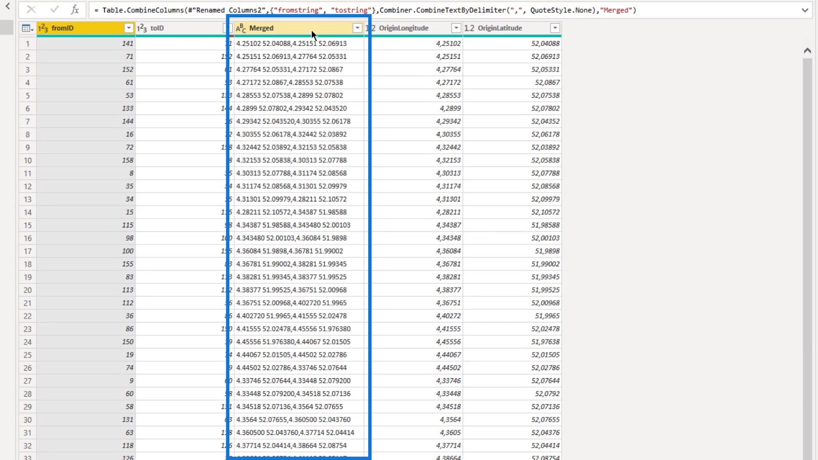
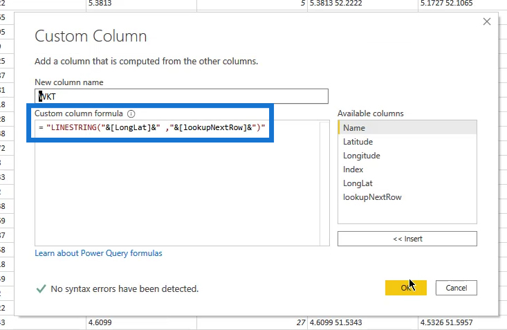
4. Creating The Well Known Text
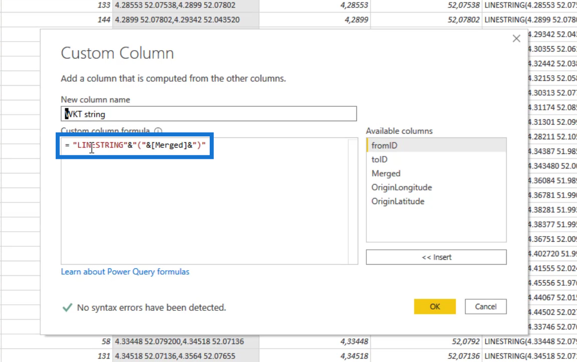
After creating the fromstring and tostring columns, I created the WKT string column.
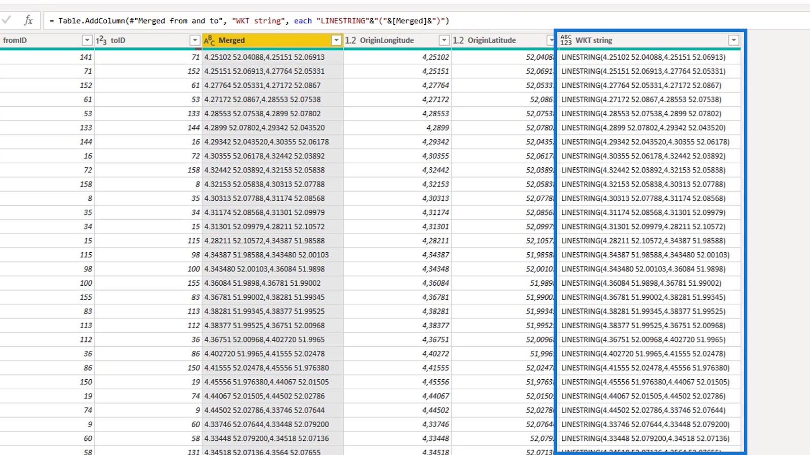
The Well Known Text is created by adding the keyword LINESTRING to the merged column.
So, it now qualifies as a Well Known Text string that will be accepted by the Power BI Icon Map Visual.
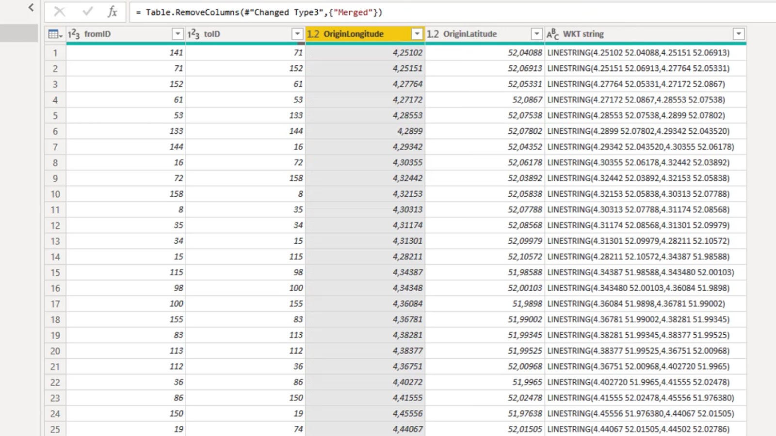
The next thing that I did was removing the merged column.
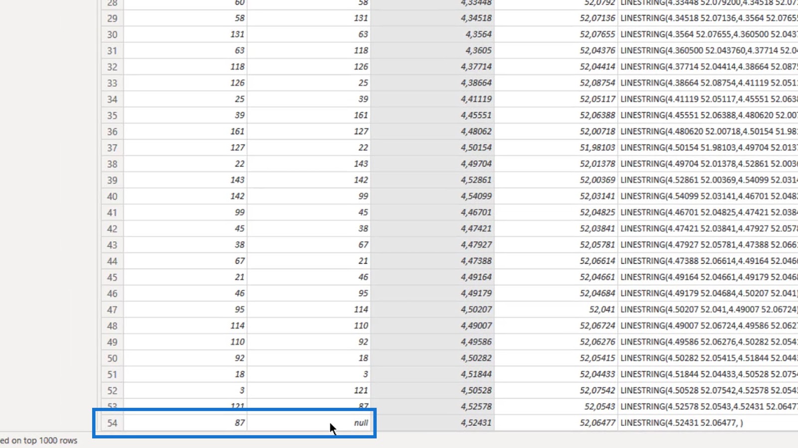
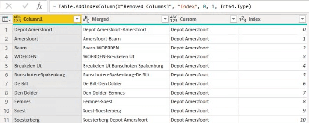
As you can see, there’s no value in the last row. This is because there’s no adjacent station. So I removed the last row.
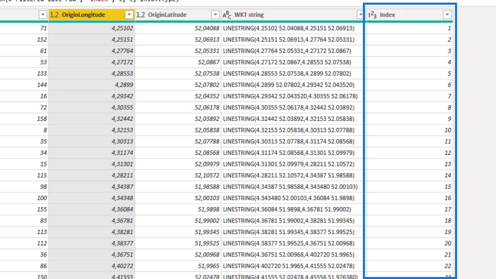
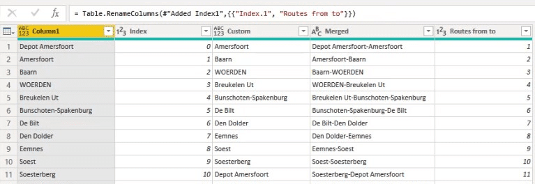
I also added an Index column for sorting the Well Known Text ID that I created in the visual.
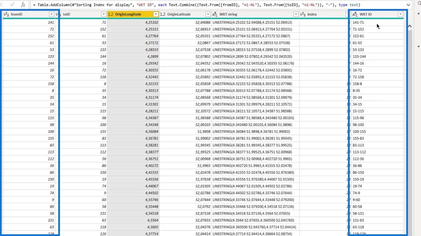
Moreover, I added the Well Known Text ID (WKT ID) column, which is a combination of the fromID and toID columns.
5. Adding A Value To Visual Data With No Value
I’d like to add a value to my visual data that doesn’t contain any value.
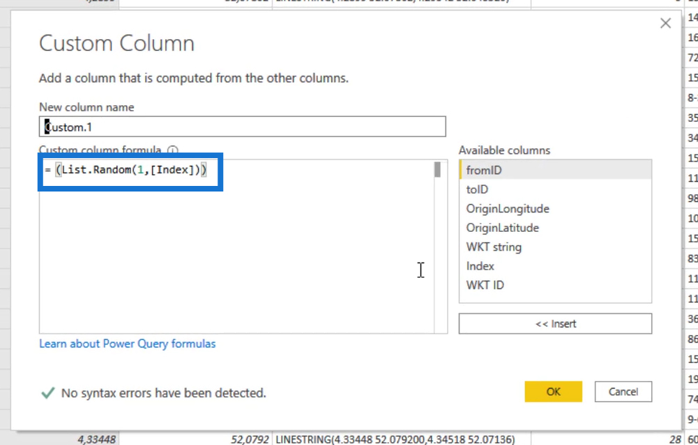
In order to do this, I created a random value column using the List.Random function and the Index column. The value could then represent the pressure, quantity, or the time without maintenance. This is just to display something in the visual.
6. Completing The Fields For The Power BI Icon Map Visual
Since I already downloaded the Icon Map visual from the website, I can simply click it here.

There’s some complexity in the usage of the visual due to the variety of available settings. I’ll quickly guide you through some of them.
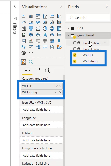
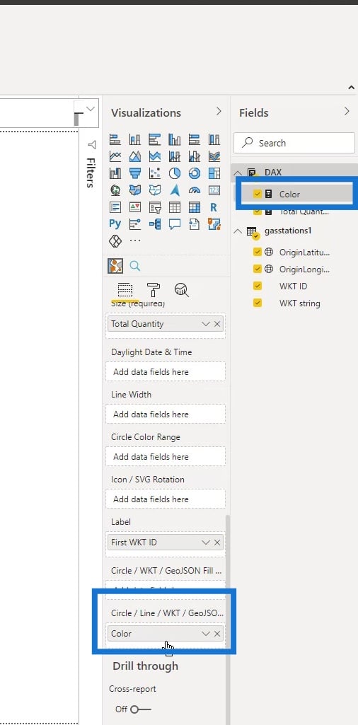
The required fields in order for the visual to work are marked as “(required)“.

To display the stations or gas lines, I added both the WKT ID and the WKT string in the Category field.
I also added the longitude and latitude.
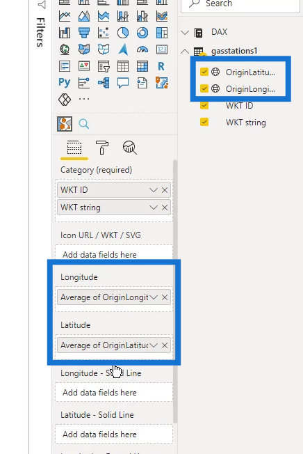
Then, I added the Total Quantities measure in the Size field.

The Total Quantities measure is the sum of the Quantity column inside the gasstations1 table.
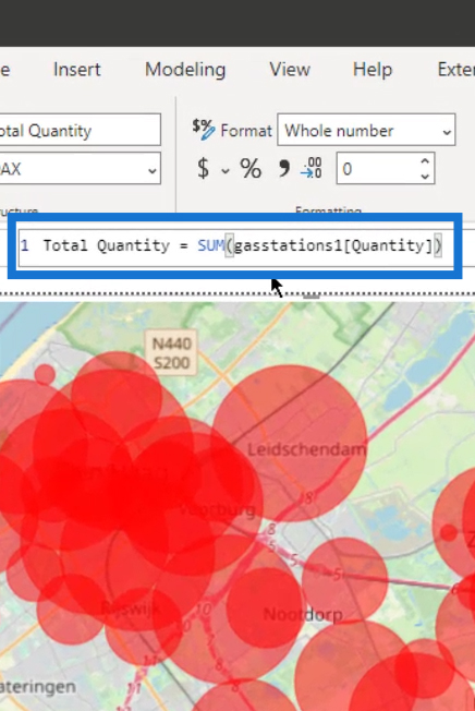
As you can see, I already have a map here. However, it’s not really what I want yet.

7. Modifying The Icon Map Visual In Power BI
I need to create some labels to make it look better. So, I placed the WKT ID column within the Label field.
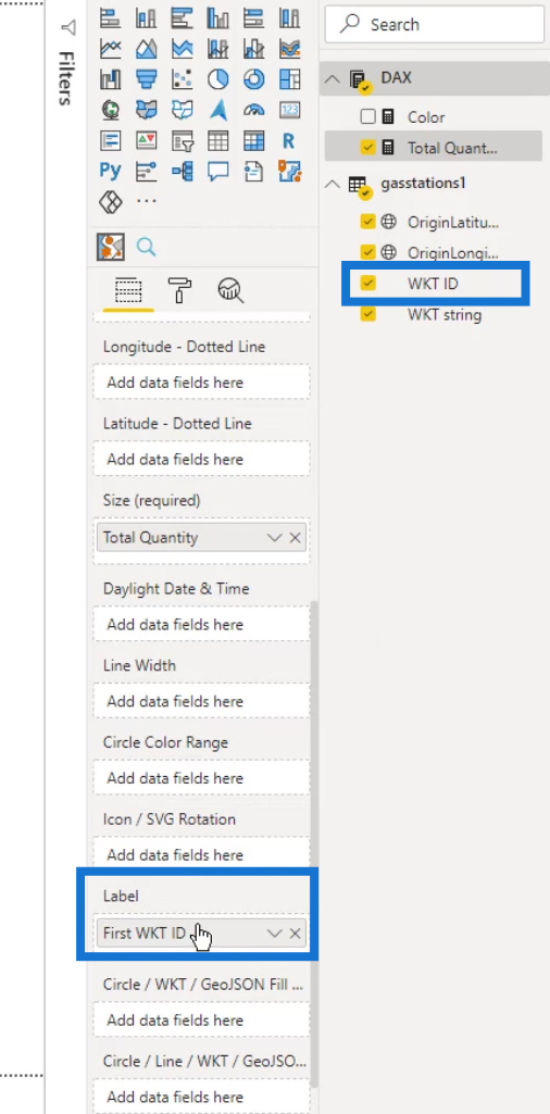
I also have a simple color measure and I’ll put it on the field here.

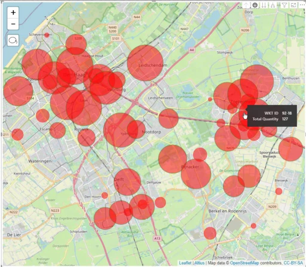
I can now use this map to display gas stations like this.
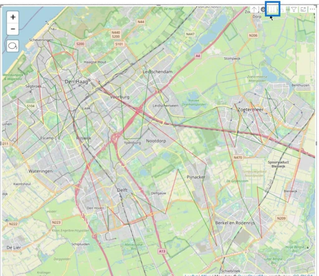
By clicking here, I can also display the layer of gas lines.
However, there are still some things that I need to do so I can make this look better.
To start, I’ll go to the Formatting pane. Then, under the Background Layers, I’ll select the Stamen – TonerLite. This provides a selection of different types of backgrounds
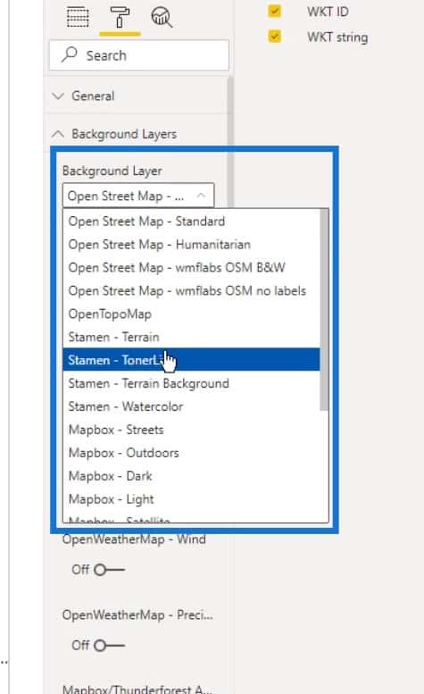
I selected this map because it’s nice and gray. It also gives a good reflection of the colors that I want to use.
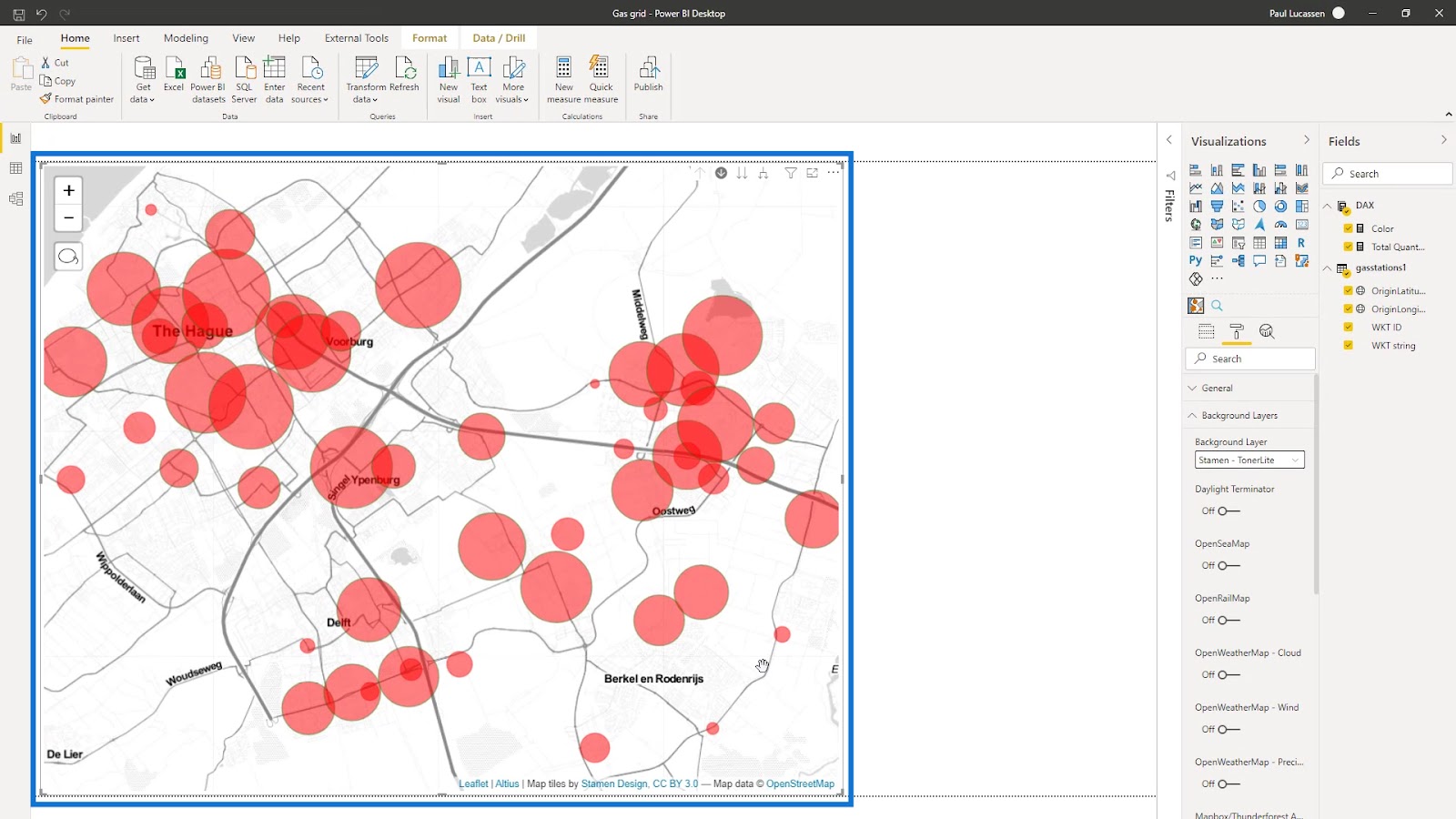
There are also different options for layers here. For instance, I’ll enable the OpenRailMap here.
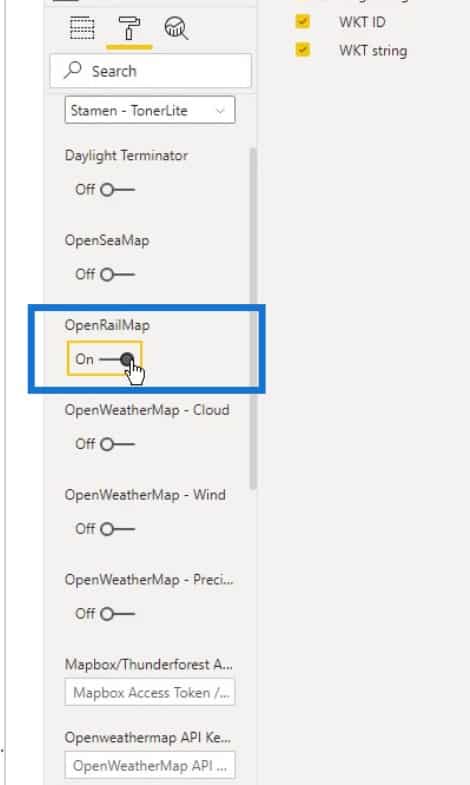
This will then add railway lines (represented in orange color) on the map.

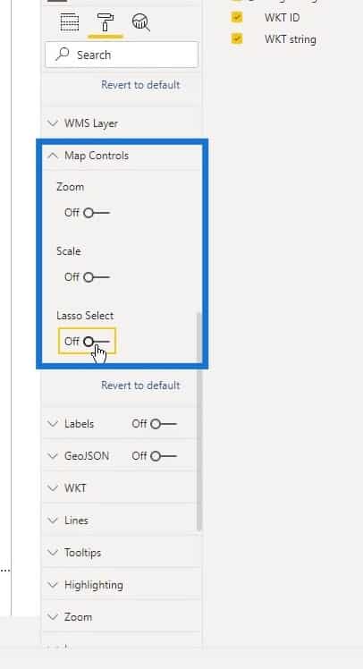
Under the Map Controls, I’ll disable the Zoom and Lasso Select options to make the map cleaner.
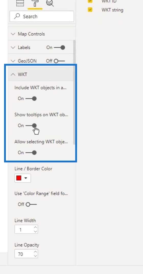
Then, I’ll turn on the Labels option here.
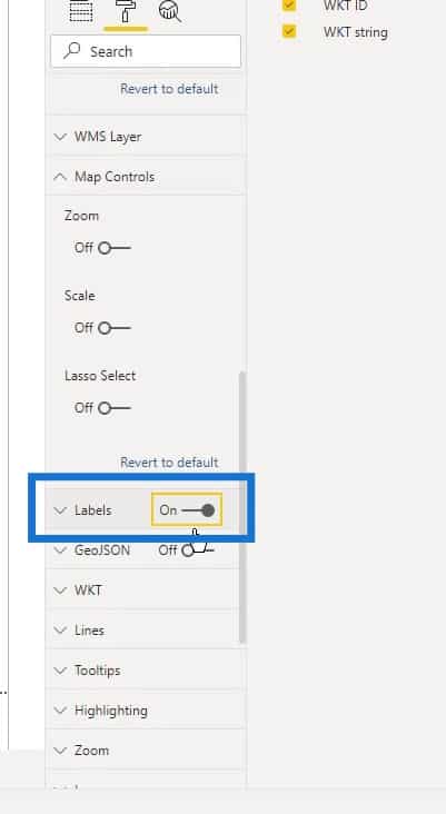
Here you can see the labels which are referring to the station or the section of the pipeline.

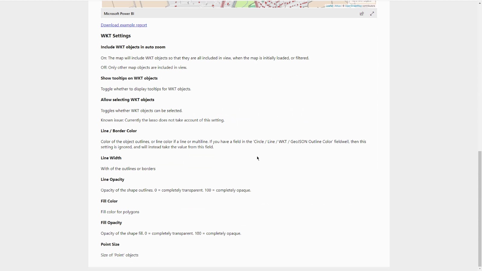
I selected all the options under the WKT as well because they also have an impact on the map display.
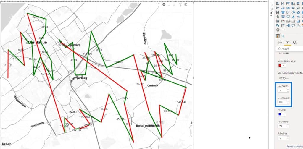
I also increased the thickness of the lines for the line layers by increasing the value of the Line Width here. Furthermore, I changed its Opacity to 100% to make it stand out.
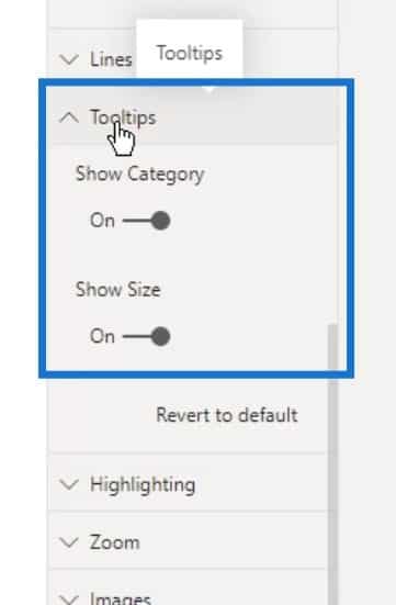
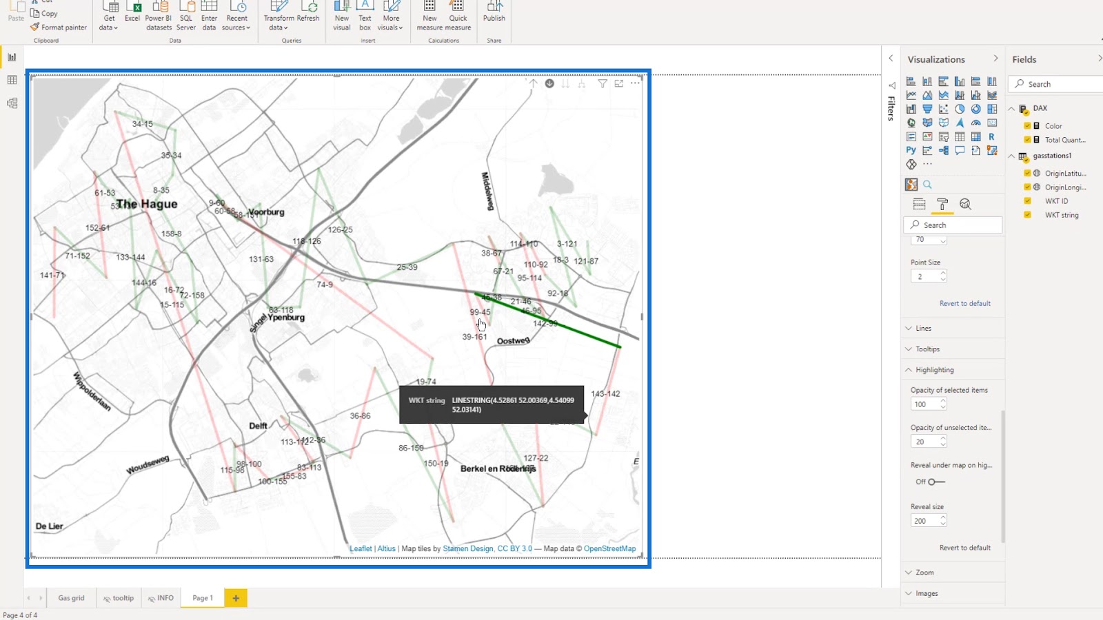
I was able to control the Tooltips here. In this example, I’ll leave it to the default setting.
Under the Highlighting, I’ve set different values for the Opacity of selected items, and the Opacity of unselected items.
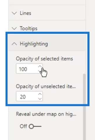
This is how it looks like when selecting one line on the map. You can see that the other lines are still visible because the opacity of the unselected is set to 20.
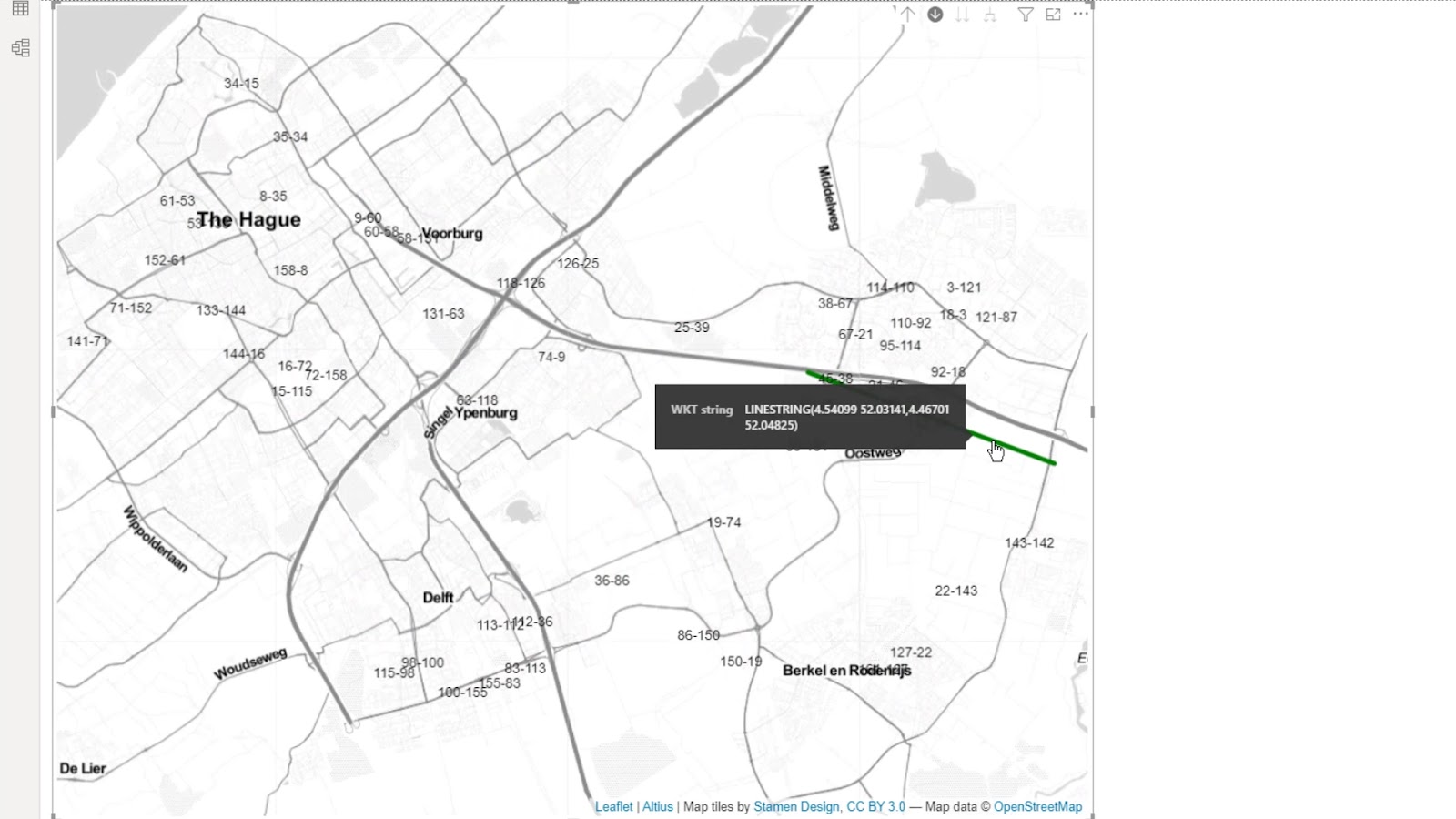
By changing the opacity of the unselected to 1, they will be completely invisible.
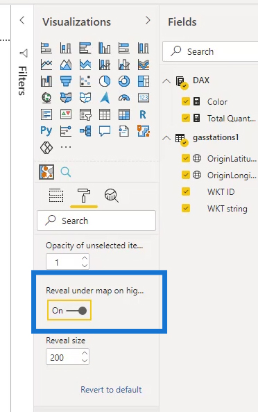
I also enabled the Reveal under map option because I might be able to use it under certain circumstances.
Then I enabled Auto zoom.

There are also other available settings that I can try and play around.

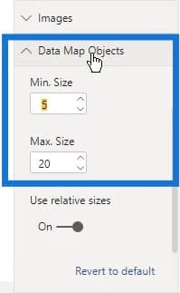
The size of these circles on the map can also be changed. Under the Data Map Objects, just change the Min. Size for the minimum size and the Max. Size for the maximum size.
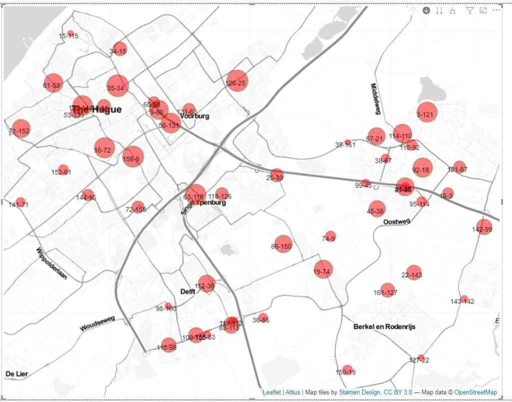
In this example, I used 20 for the maximum size, and 3 for the minimum size.
8. Adding A Tooltip
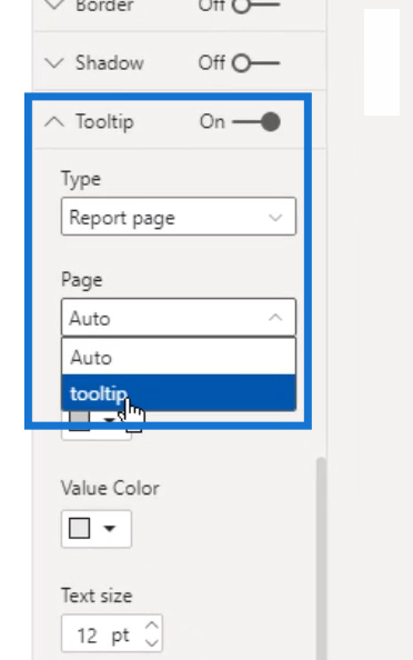
I created a simple tooltip that looks like this.

I was able to use that tooltip here. Under the Type option, I selected the tooltip option which is the name of the tooltip that I created. Note that this Tooltip option here is different from the Tooltips that I previously mentioned.
After that, as I hover over my map, you can see the tooltip that I created.
Depending on the map that you are creating, the other settings might not be relevant. As you can see, the settings might be overwhelming, but they all contribute to a better map appearance.
9. The Output
Now, I have a map that can show multiple layers. I can switch between the stations that I can display as circles or lines.
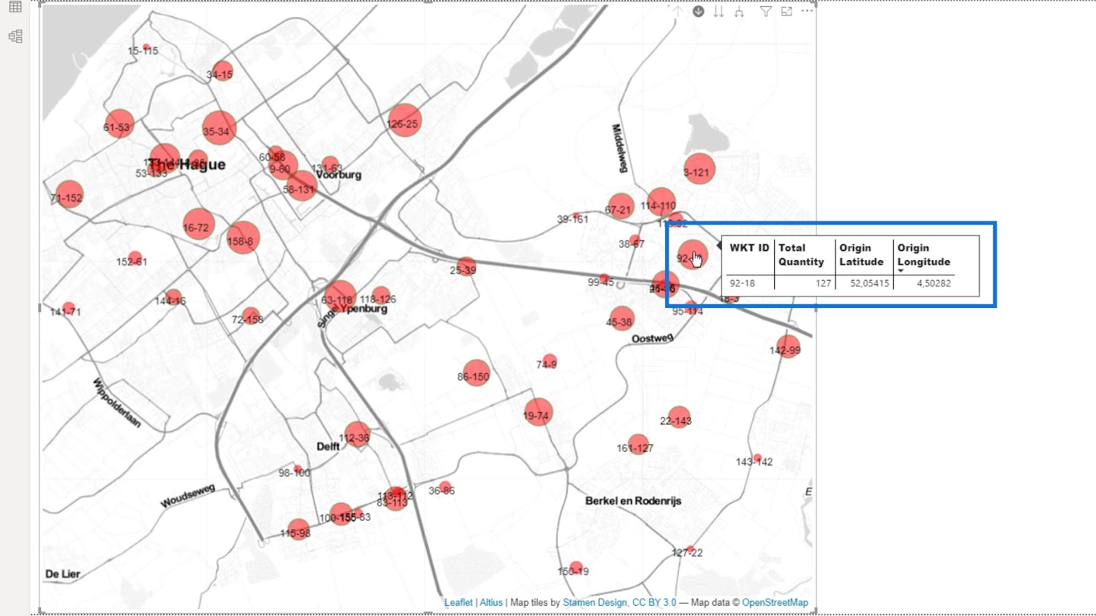
After completing the previous steps, it’s now possible to add a table to reflect the selections that you are making in the map.
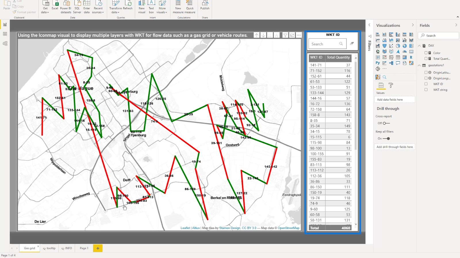
In this example, I can select a point here, and it will show that point on the map.
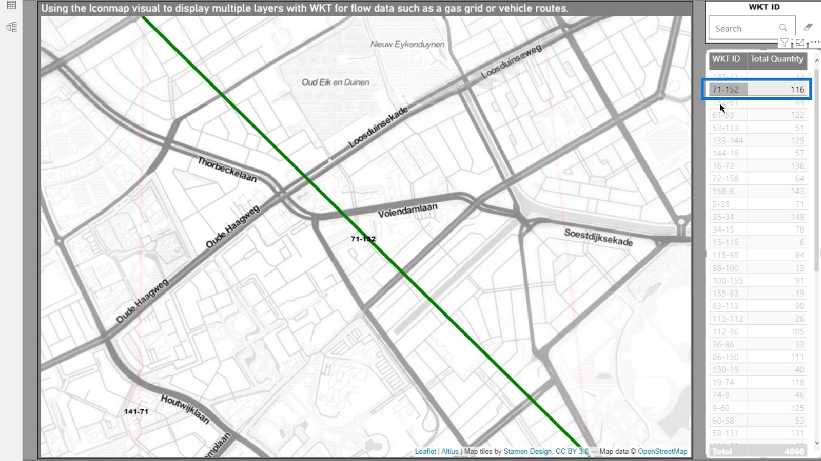
I can also use the search feature here. For example, If I type 61, it will also show those points on the map.

Lastly, I can just select an item on the map by just clicking on it. Then, it will be displayed on the table.

That wraps up the first part of this Well Known Text tutorial.
Sample Power BI Icon Map Scenario Based On Delivery Routes
In this second example, I’m looking at delivery routes. Again, most of the work is done in Power Query. The way I handled the data in the first example is not very different from what I used in this example. But I still have completely different data in this example.
In this second example, I want to analyze the routes from several vehicles that are from varying depots. Then, display them as straight lines connecting the from and to locations in each delivery route.
Depending on what is available in your data, you could analyze the emission per stop, the fuel consumption, the stop time, and many more. This example will only show weight and revenue.
One of my current projects seeks to calculate the emissions across multiple type of vehicle routes and the various circumstances. This required a transportation tender response.
1. The Dataset
The data that I used originated from a transport management system. There are various ways that data may become available. They can be from different types of transport management systems, from a route optimization program, or from a board computer.

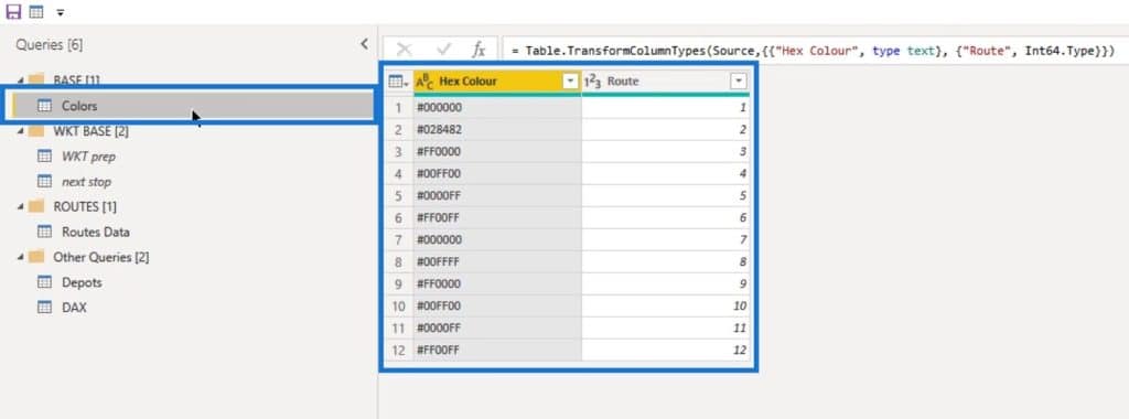
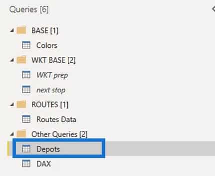
In the Power Query, I currently have five queries. First is a Colors table to control the color display for the routes.
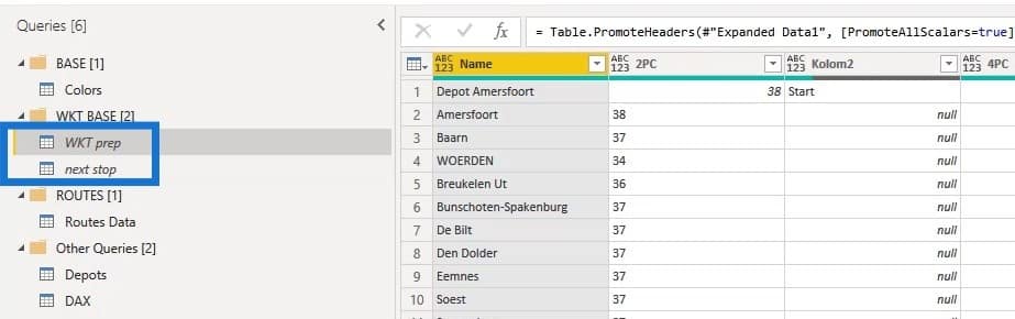
I also have two queries that are duplicates of the Routes Data query with part of the Power Query data transformation. I named them WKT prep (Well Known Text Preparation) and next stop (Next Stop Preparation). These two are used to merge the required information with the main Routes Data query.
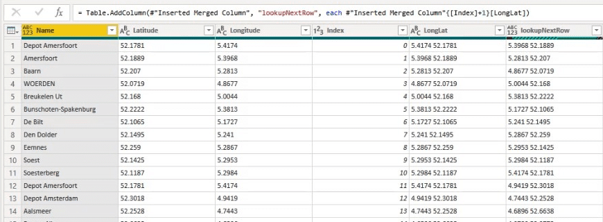
There are a few ways on how to complete one of the key requirements in this case. And that is getting the name, the latitude, and the longitude of the next row into the previous row to show the sequence of the delivery.
Next is to show the departing and arriving depot in the correct columns.
Lastly, I created a Well Known Text string.
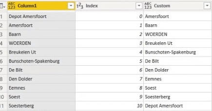
I used both the index methods and merging with shifted indexes zero to one or one to two to align the records. I also utilized a custom column solution where the index number plus 1 will return the next row.
This may incur memory issues in bigger datasets.
So, using the methodology to merge based on the index column is preferable as it is much more simple.
I also have the Routes Data query. This will be loaded into the model.
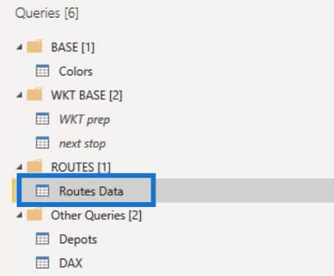
The Depots query contains information regarding the start and endpoint of each route. I also merged this query with the Routes Data query.
The model and underlying data will be available for reference. I suggest walking through the applied steps at your own pace from merging the Depots query to get the latitude and longitude. Then proceed to the step for the next stop merging in order to add the Well Known Text to the data. After that, you can move on to doing the steps for final cleanup.

I loaded the Depots, Colors, and Routes Data tables. I also created a connection in the data model.

So, I can now start with the visualization.
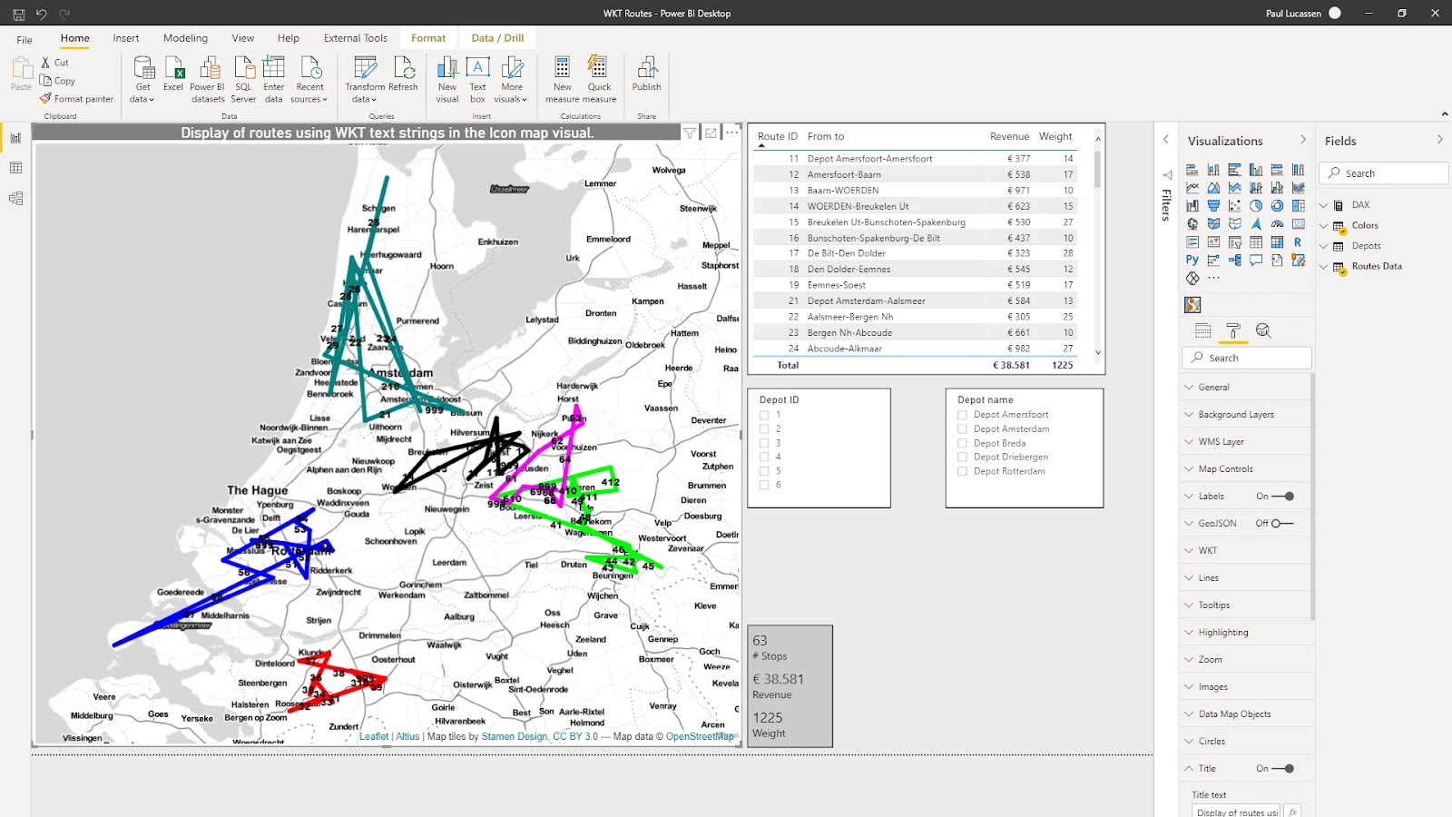
2. Icon Map Visualization
The Icon Map visual now shows the routes. It also added the relevant data into the fields row. The settings in the Formatting pane are similar to the settings in the first example which shows the gas stations.
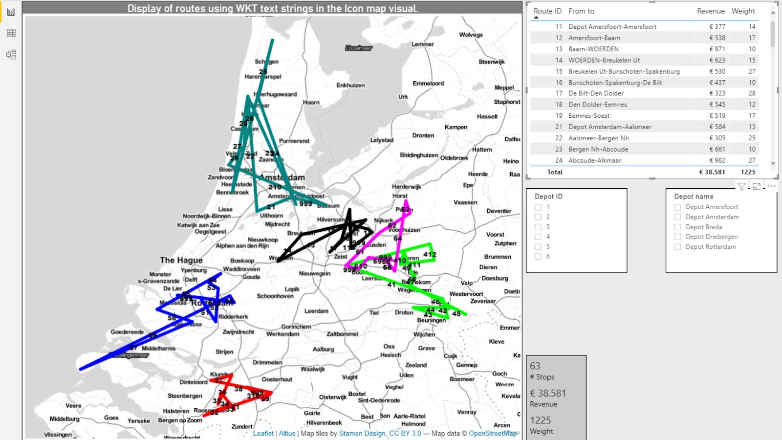
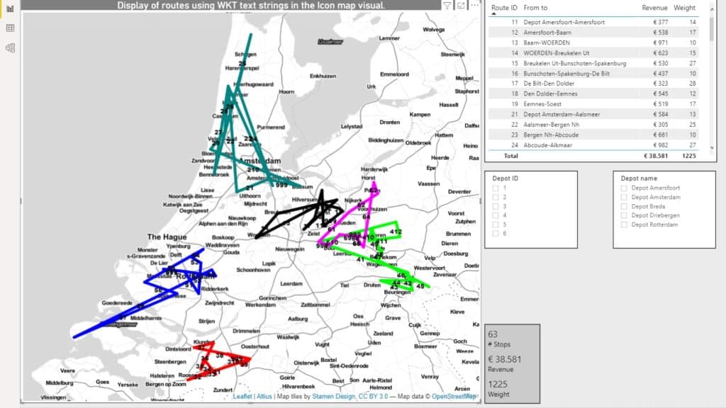
I added a few measures to calculate the number of Stops in the routes, the Revenue, and the Weight. These were placed in the cards.
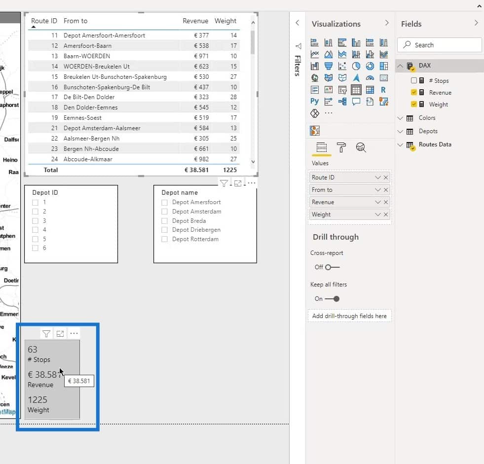
After adding a table and slicers for the Depot ID and Depot name, the basic route analysis dashboard is completed. This is now dynamic as I can make the selections that I want and the results will display accordingly.

***** Related Links *****
Data Visualizations Power BI – Dynamic Maps In Tooltips
Power BI Shape Map Visualization For Spatial Analysis
Geospatial Analysis – New Course on Enterprise DNA
Conclusion
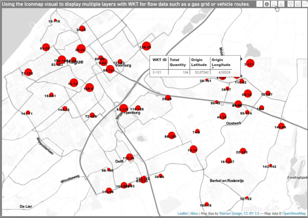
That is basically how to use well-known text strings in a Power BI icon map visual. In this tutorial, you were able to learn how to display multiple layers with WKT for flow data such as a gas grid or vehicle routes in the icon map visual.
Keep in mind that adding the relevant and required data fields are also essential to make the analysis report properly work.
Check out the links below for more examples and related content.
Cheers!
Paul