How to Multiply Two Columns in Excel

Mastering essential Excel functions is a critical part of a data-driven world, and one of those crucial functions is the ability to multiply two columns in Excel.

This tool is often used in various business and scientific scenarios to calculate total sales, revenue from multiple sources, or any interactive model.

To multiply two columns in Excel, individual cells can be multiplied by using the “asterisk symbol. For example, to multiply a value in cell A2 with the respective value in B2, you can enter “=A2B2″ in a new cell.

This process is crucial but not often covered in common Excel tutorials. In this article, we’ll go through the steps with practical examples and use cases to help you understand better.

Let’s get started!

Understanding the Basic Operators in Excel

Excel is equipped with simple arithmetic operators to perform basic calculations.

Investing a little time to familiarize yourself with these basic operators will help you complete your tasks efficiently and effectively.

Furthermore, you’ll find that even as you progress to more complex tasks, the fundamental arithmetic operators in Excel are crucial.

There are a few basic arithmetic operators in Excel that we will define below:

• Addition (+): This operator performs addition on two or more numbers. Example: 5+3 equals 8.

• Subtraction (-): This operator calculates the difference between two numbers. Example: 8-3 equals 5.

• Multiplication (*): This operator performs multiplication on two or more numbers.

This article will use the multiplication operator to multiply values from separate columns.

• Division (/): This operator calculates the quotient of two numbers. Example: 8/2 equals 4.

To understand the above operators better, we have shown it in the below example:

Different Ways to Multiply Two Columns in Excel

There are several methods available to multiply two columns in Excel. Each approach has specific use cases, but remember to choose the one that best suits your needs.

Let’s dive into the basics and get familiar with some key methods for achieving this task.

1. Using “*” (Asterisk) Symbol

The most common method to multiply two columns in Excel is by using the multiplication operator.

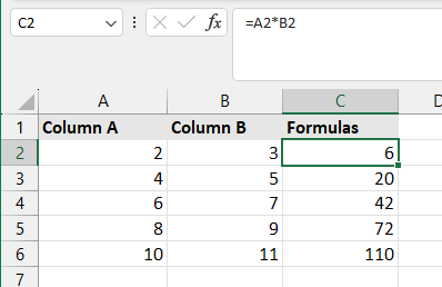
In this example, the formula multiplies each cell from column A with the corresponding cell in column B.

When you press ENTER, Excel will multiply cell A2 by B2 and display the result in cell C2.

To apply the formula to all subsequent rows, you can click and drag the bottom-right corner of cell C2 down to cell C5.

This will extend the formula to all rows, and Excel will efficiently multiply the values from columns A and B.

2. Using the “PRODUCT” Function

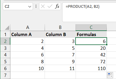
• Select the cell where you want your final value.

• Type =PRODUCT(first_cell, second_cell), the asterisk symbol (*) can represent all cell addresses without any comma in between.

• Press the Enter key.

• As shown below, click and drag the fill handle down to other rows.

This will apply the PRODUCT function to all rows, multiplying all numbers in each row and then summing up two columns.

The PRODUCT function efficiently utilizes relative cell references, especially when dealing with many rows.

This will combine the values into a single cell and multiply two in the same cell in Excel.

Multiply Columns Using the Paste Special Feature in Excel

In many business scenarios, you might encounter situations requiring you to multiply data in one column by numbers or percentages in other columns.

One indispensable feature in Excel is the Paste Special option, which offers five operation types: Add, Subtract, Multiply, Divide, or Power.

This functionality allows you to perform arithmetic calculations between the copied data and the destination cells without the need for complex formulas or functions.

Let’s look at how to use the Paste Special options.

let’s focus on a scenario where we want to copy the Net Income values without the underlying formulas. Here’s how you would do it:

1. Calculate Net Income: The table already includes a “Net Income” column, calculated as Profit * (1 – Tax Rate). The profit is the difference between profit, revenue, and cost.

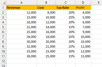
2. Copy the Net Income Values: Click on the top cell of the Net Income column in the table (let’s assume it’s in column E, starting from cell E2). Then, drag down to select the entire Net Income column up to the last row of your data (e.g., E2 to E11).

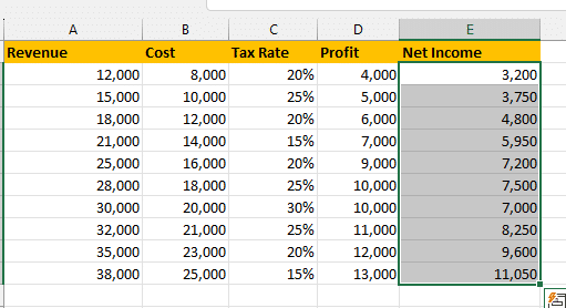
3. Use Paste Special for Values:

To increase the Revenue by 10% using Excel’s Paste Special feature:

1. Copy the “Percentage Increase” column (which contains the value 1.10 for each row).
2. Select the “Revenue” column.
3. Right-click on the first cell of the “Revenue” column and choose “Paste Special.”

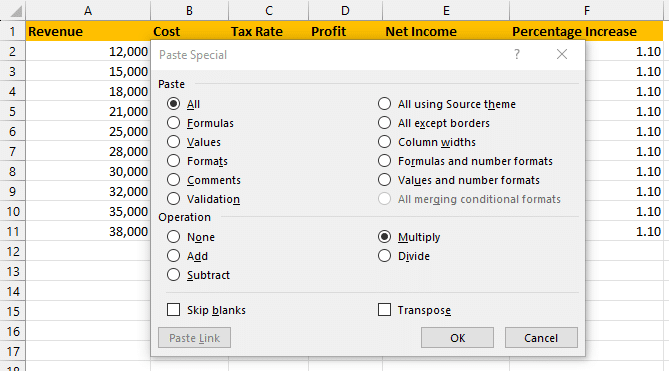
4. In the “Paste Special” dialog box, select “Multiply” under the operation section, and click “OK.”

5. This process will multiply each Revenue value by 1.10, effectively increasing each value by 10%.

By implementing this method, you can streamline the process of multiplying columns in Excel while maintaining flexibility for various business applications.

Let’s look at another popular method for multiplying columns, indexes, and matches.

How to Multiply Columns Using INDEX and MATCH in Excel

Excel is a powerful tool for data analysis, and the INDEX and MATCH functions are critical players in data lookup scenarios. The INDEX and MATCH formula combination allows you to search for a value in a table and return its row or column number.

The INDEX and MATCH functions are commonly used together for complex lookups in Excel. Here’s a simplified explanation of how they work:

• MATCH: This function searches for a specified item in a range of cells and then returns the relative position of that item. For example, MATCH(“Apple”, A2:A10, 0) would search for the word “Apple” in the range A2:A10 and return its position in that range.

• INDEX: This function returns the value of a cell in a specific row and column of a range. For example, INDEX(B2:B10, 3) would return the value in the third row of the range B2:B10.

To multiply values from two columns based on a lookup, you can combine these functions. Let’s consider a practical example using a simple product table:

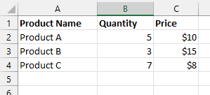
Suppose you want to find the total cost for a specific product by multiplying its quantity by its price. You can use INDEX and MATCH to determine the product’s price and multiply it by quantity. Here’s how you can do it:

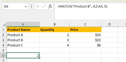
1. Create a Lookup Formula: Assume you want to find the total “Product B” cost. You would first find the row where “Product B” is located using MATCH: MATCH(“Product B”, A2:A4, 0). This would return the relative position of “Product B” in the range A2:A4.

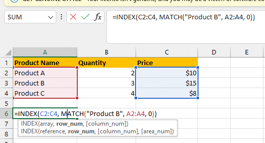
2. Retrieve the Price: Next, you use INDEX to find the price of “Product B”: INDEX(C2:C4, MATCH(“Product B”, A2:A4, 0)). This formula looks up the price in column C corresponding to “Product B”.

3. Multiply with Quantity: Finally, you multiply this price by the quantity of “Product B”, which is in another column (let’s say B2 for “Product A”, B3 for “Product B”, and so on). The complete formula in a new cell would be =B3*INDEX(C2:C4, MATCH(“Product B”, A2:A4, 0)).

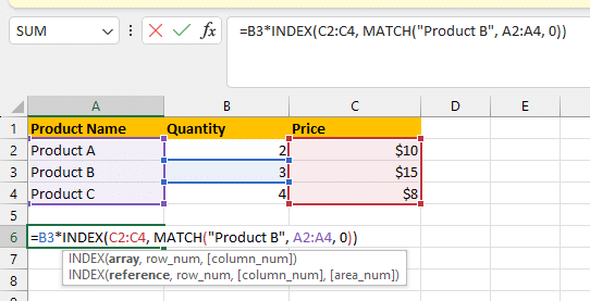
This formula will give you the total cost for “Product B” by multiplying its quantity (from column B) by its price (looked up using INDEX and MATCH in column C).

Now and then, you’re bound to run into some issues. Check this next section to help you diagnose and overcome them.

HoProfitandle Error Messages and Blank Cells

While multiplying columns in Excel, you may encounter error messages or blank cells. However, in such scenarios, there are techniques that you can use to handle these issues effectively and ensure accurate results in your calculations.

Here are some common occurrences and how you can manage them:

1. Addressing #DIV/0! Errors

The #DIV/0! error occurs when the divisor in your formula is zero. For example, dividing a number by zero will result in this error.

Excel does not allow division by zero due to mathematical impossibility.

To fix this, you can wrap the formula within an IFERROR function. This function will check for errors and return a specific value if found.

For instance, to handle the #DIV/0! Error in a multiplication formula, use the following pattern:

The formula checks if a divisor, in this case, the cell C1, is zero. If it is, it will display “N/A” (or any other specified text) instead of a 0.

2. Dealing With Blank Cells

When your data contains empty or blank cells, it may negatively impact the accuracy of your calculations. To handle this, there are a few options you can consider:

• Use the IF function to replace the blank cell with a default value. For instance, if A1 is blank, you can replace it with 1 using the formula: =IF(ISBLANK(A1), Default_Value, A1)

• Use the PRODUCT function, which skips over blank cells by default, to perform multiplication on entire columns without the need to adjust for blank cells.

• Filtering out blank cells is another option: using the FILTER function to remove all the rows with a blank cell.

• Replace blank cells with zero: You can perform calculations without worrying about affecting the results. Consider replacing blank cells in a new column with a default value 0.

Let’s reflect on some final thoughts.

Final Thoughts

After reading this article, you should feel more confident about mastering the technique for multiplying two columns in Excel. Understanding and implementing this process can significantly enhance your skills and efficiency in manipulating data.

Once you become adept at this fundamental task, you’ll find that your productivity increases as you tackle more complex tasks. Regular practice and trying new Excel features as they are released will help reinforce your knowledge and skills.

If you’d like to learn about Power BI and how it can greatly enhance your data analysis skills, check out the video we’ve prepared for you below:

Frequently Asked Questions

Can the Power Query Editor Multiply Different Columns?

The Power Query Editor is a versatile tool that allows you to manipulate and transform your data by applying a wide range of operations. Multiplying columns in Power Query is both possible and straightforward.

To multiply columns in Power Query, follow these steps:

1. Load your data into Power Query by clicking “Data” and then “Get Data”.

2. In Power Query, select “Combine and Edit” from the home tab.

3. In the editor, add a new custom column.

4. In the formula area for the new column, enter a formula to multiply the columns. For example, if you want to multiply ‘Column1’ by ‘Column2’, the formula would be [Column1] * [Column2].

5. The result column will display the product of the two selected columns for each row.

This method is helpful for tasks like recalculating overall revenue or adjusting prices by a particular factor. The computed values remain up-to-date and reflect changes in the source data.

How do you use the INDEX Function to Multiply Columns?

In Excel, the INDEX function returns the value of a cell in a table based on the intersection of a specified row and column. You can use the INDEX function to multiply values from two columns. For example:

1. To multiply individual cells in columns A and B, use: =INDEX(A:A, ROW()) * INDEX(B:B, ROW()). This formula multiplies corresponding cells in columns A and B.

2. To multiply entire columns, use array formulas or iterative methods, as Excel does not support direct full-column multiplication using the INDEX function.

Does the SUMPRODUCT Function Depend on Cell References?

The SUMPRODUCT function in Excel multiplies items in two or more arrays (ranges) and then sums the results. It is a versatile and efficient function for array operations.

For example, to compute total revenue by multiplying ‘Price’ in column A and ‘Quantity Sold’ in column B, use: =SUMPRODUCT(A2:A5, B2:B5). This formula multiplies each price in A2:A5 by its corresponding quantity in B2:B5 and sums these products.

The function can use cell references, like A2:A5 and B2:B5, ensuring dynamic calculations that adapt to changes within the range. The formula remains concise and efficient for multiplying and summing values.