When working with Microsoft Excel, you may occasionally encounter what is known as a circular reference. This is when a formula in a cell refers back to itself, causing an endless loop in the calculation process.
To find circular references in Excel, use the “Error Checking” tool under the “Formulas” tab to identify cells with a circular dependency.
This article shows you how to find circular references in Excel and fix them. You will also learn how to prevent them when working with large or complex worksheets.

What Are Circular References
Circular references occur in Excel when a formula calculation in a cell depends on the cell’s own value. This creates a loop and leads to incorrect or unpredictable results.
This is easier to understand with a simple example.
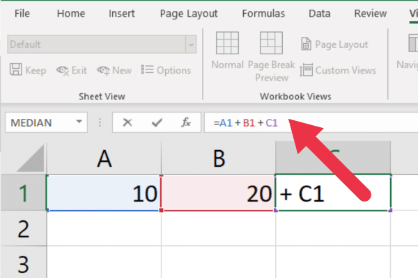
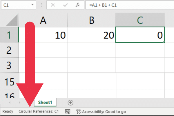
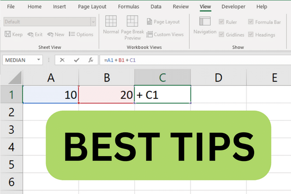
Suppose you have two numbers in cells A1 and B1. You want to use a formula in cell A3 that adds the two numbers together. The formula in cell A3 should look like this:
=A1 + B1
However, if you make a mistake and include C1 in the calculations, you now have a circular reference:
=A1 + B1 + C1

This may be an obvious problem to avoid when dealing with two cells. However, when you are working with large ranges of cells, mistakes become more likely.
Thankfully, Excel is designed to handle such situations by displaying a warning message when a circular reference is detected.
However, in some cases, you might encounter a circular reference without receiving any alert. Therefore, it is important to know how to find and resolve these issues manually.
The Circular Reference Error Message Window
By default, Excel monitors for circular references as you enter formulas into cells. When you press enter in a cell with a problem, a pop-up window will display the circular reference error message.
This is the explanatory text:
There are one or more circular references where a formula refers to its own cell either directly or indirectly. This might cause them to calculate incorrectly. Try removing or changing these references or moving the formulas to different cells.
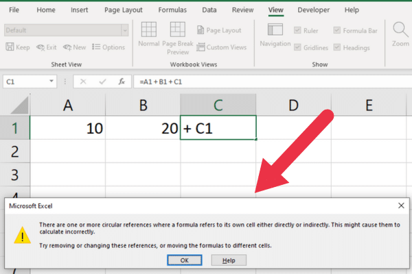
When you see this dialog box, you should click “OK” and use the methods in this article to fix the problem.
However, you don’t need to fix the error immediately. You can continue working with the spreadsheet with the intention of resolving the problem later.
In that case, you need to know how to find circular references in Excel after you’ve dismissed the warning box.
How to Find Circular References in Excel
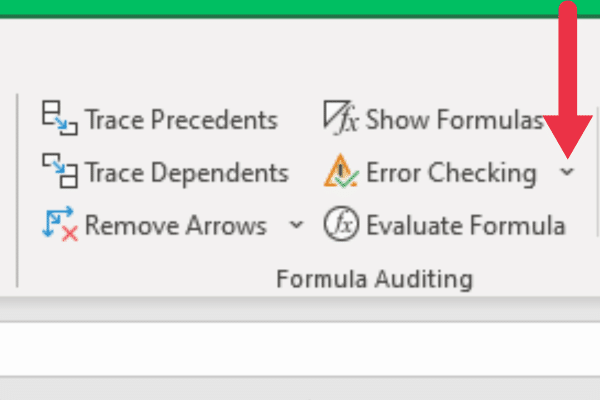
Excel has a built-in error checking tool that finds several kinds of errors, including circular references. You access the tool on the Formulas tab.
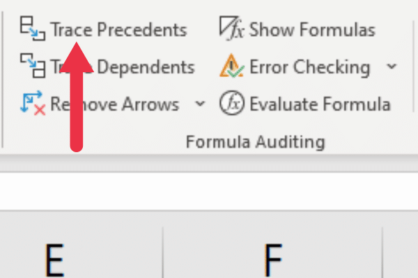
This picture shows the location within the Formula Auditing group.
Now you know how to find the tool, here are the detailed steps to use it:
1. Go to the Formulas tab.
Click on the Error Checking drop-down in the Formula Auditing group.
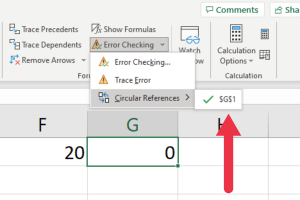
Select “Circular References” from the dropdown list.
Click the link to jump your cursor to the first cell with an issue.
The picture below shows that the tool has found a circular error in cell G1. The displayed cell is a hyperlink.
When you click the link, your cursor moves to the cell. This is very helpful with a large volume of data.

Once you’ve resolved the first circular reference, you can go back to the Error Checking tool to find the next one on the sheet.
Use the steps in the later sections of this article to fix the issue and use the tool to go to the next problem.
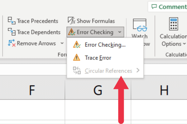
If there are no more circular issues, the “Circular References” menu item in the drop-down menu will be grayed out. You have no further work to do.
How to Find Circular References With The Excel Status Bar
Another way to spot a circular reference is to look at the status bar at the bottom of the Excel worksheet.
When there are one or more issues in the worksheet, the status bar displays the location of one problem cell reference.
For example, if there is a circular reference in cell C1 and there are no other issues with the spreadsheet, the status bar will read: “Circular References: C1”.
This picture shows you where to see the display.
How to Find Hidden Circular References In Excel
Hidden circular references in Excel are circular references that are not immediately detected by the in-built error features. In other words, Excel does not display the standard warning.
They happen when a cell references another cell indirectly, through a series of intermediate cells, and eventually refers back to the original cell.
Excel has two tools that help you trace relationships and investigate these issues:
Trace Dependents tool
Trace Precedents tool
How to Use The Trace Dependent Tool
Experienced Excel users take advantage of the Trace Dependents tool to investigate these issues and fix circular references. By choosing one or more cells and using this tool, Excel will show you the dependent cells.
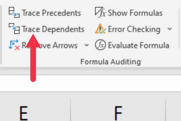
The tool is available in the Formula Auditing section on the Formulas tab.
To use the tool, follow these steps:
Click on the cell or cells you want to trace dependents for.
Go to the ‘Formulas’ tab in the Excel ribbon.
Click on the ‘Trace Dependents’ button in the ‘Formula Auditing’ group.
Review the tracer arrow or arrows showing dependencies.
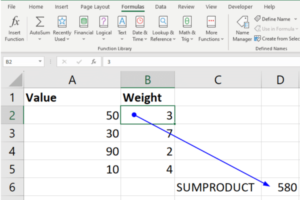
Excel shows arrows from the active cell value to any cells that depend on it. The blue arrow in the picture below shows that cell D6 has a dependency on cell B2.
Trace Precedents tool
Precedents are the opposite of dependents. The Trace Precedents tool lets you pick a cell with a formula and see all the cells that it depends on i.e. the precedents.
The tool is available in the Formula Auditing section on the Formulas tab.
To use the tool, follow these steps:
Click on the cell containing the formula you want to investigate.
Go to the Formula tab in the Excel ribbon.
Click on the ‘Trace Precedents’ button in the ‘Formula Auditing’ group.
Review the trace arrows that Excel displays.
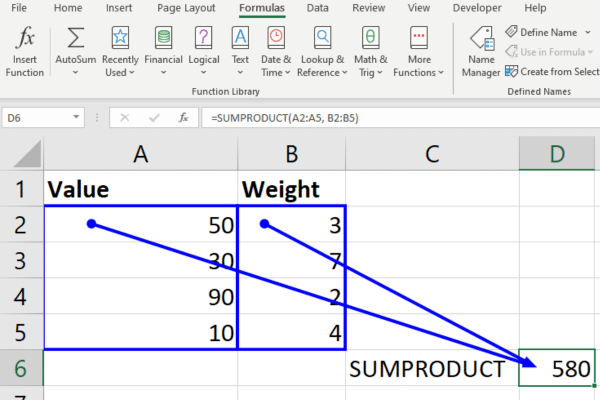
The blue arrows in the picture below shows you that cell D6 is dependent on the range of cells A2:B5.
Using both tools helps you find Excel circular references that are not immediately apparent. The next step is to fix the problem in the selected cell. You can then continue to search for the same problem in other cells.
2 Ways How To Remove Circular References In Excel
There are two main methods to resolve circular references:

breaking the circular reference
using alternative formulas
Let’s explain both ways.
1. Breaking the Circular Reference
Breaking the circular reference in Excel is an efficient way to resolve the problem. This requires you to identify the cells involved in the circular reference and modify their formulas accordingly.
To do this, follow the steps described earlier to find the cell address.
You should then examine the formula in the Formula Bar. Look for a reference to the cell itself.
In our first example of a circular reference, the addition formula in cell C1 included a reference to the cell itself:
=A1 + B1 + C1
This can be fixed by removing the final addition. Once this problem is resolved, you move on to find other circular references and address them.
2. Use Alternative Formulas
Some of the most common causes of circular references are when summing or averaging cells. The mistake is to include the results cell in the formula.
In our previous example, the formula used addition operators to calculate the sum of a range of cells. The alternative method is to use the SUM Excel function.
To fix the example, you replace the formula with:
=SUM(A1:B1)
Similarly, you could average a range with a formula like =(A1+B1)/2. However, the AVERAGE function is less likely to lead to a mistake.
=AVERAGE(A1:B1)
5 Tips For Preventing Circular References
To prevent circular references in Microsoft Excel, it’s essential to have a clear understanding of how your formulas interact with each other in your Excel sheet.
By identifying the relationships between cells and being aware of how these connections work together, you can avoid creating circular formulas.
Here are our five best tips to help you prevent circular references.
1. Be Careful When Selecting Ranges
In my experience, one of the most common causes of circular references is when users are quickly selecting ranges to include in their formulas.
When swiping vertically and/or horizontally to group cells, it’s easy to select one more cell that is adjacent to the correct range. If that cell is also the results cell, you have inadvertently created a circular reference.
This mistake is typically made when working with large sets of data, such as running chi-square tests. The solution is to be careful with your range selection.
2. Plan your formulas carefully
Before entering formulas, think about the logic behind your calculations and how they should flow across cells.
You can map out the calculations in advance using diagramming tools or a whiteboard.
This can help you identify any possible loops that might lead to circular references.

3. Use alternative formulas
Certain functions, such as INDIRECT or OFFSET, can inadvertently create circular references when used improperly.
Consider using alternative functions that provide similar functionality without the risk of circular references.
4. Break complex formulas into smaller parts
Instead of creating a single complex formula with multiple nested functions, consider splitting your calculations into smaller, more manageable parts.
This not only makes your workbook easier to understand and maintain but also reduces the chances of introducing a circular reference.

5. Fix problems as you go
When working with large or complicated workbooks, it’s also essential to monitor for circular references. Instead of ignoring issues until a large set of data and formulas has been assembled, it’s better to fix each error as it arises.
You may choose to ignore a circular reference warning message for a short while. However, you should use the Error Checking feature to catch up with the existing circular references before too long.
This makes them easier to fix and preventing their effects on your workbook.
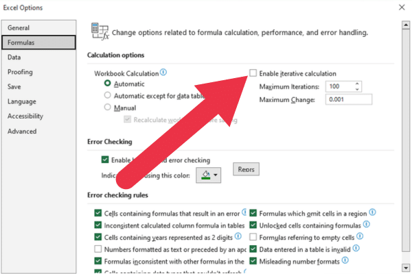
How to Enable Iterative Calculation & Why Bother?
You usually want to avoid circular references in your worksheet. However, there are some scenarios where they are necessary.
For example, some engineering or scientific calculations need to use the result of a previous calculation. This is known as an iterative solution.
Each loop refines the results of a calculation until a specific threshold or target is reached.
In these cases, it’s essential to enable Iterative Calculations in the Excel settings to allow intended circular references. This allows the software to repeat the calculations a specified number of times, converging to a solution.
Follow these steps to make a circular reference work in your Excel file:
Click the File tab.
Select Options.
Choose the Formulas category.
Under the ‘Calculation options’ section, check the box for ‘Enable iterative calculation’.
Change the number in the maximum iterations box or leave as the default of 100.
Use the maximum change box to reduce iterations as per your requirement.