This blog will teach you how to break down Power BI time series data into essential components. You can watch the full video of this tutorial at the bottom of this blog.
Time series data is everywhere, from heart rate measures to unit prices of store goods, and even in scientific models. Breaking this data into essential parts can be advantageous, especially in preparing report charts and presentations.
This blog’s time series decomposition method will help you find a better way to present data when describing trends, seasonality or unexpected events. It’s also a great stepping stone for forecasting in Power BI.

Types of Graphs
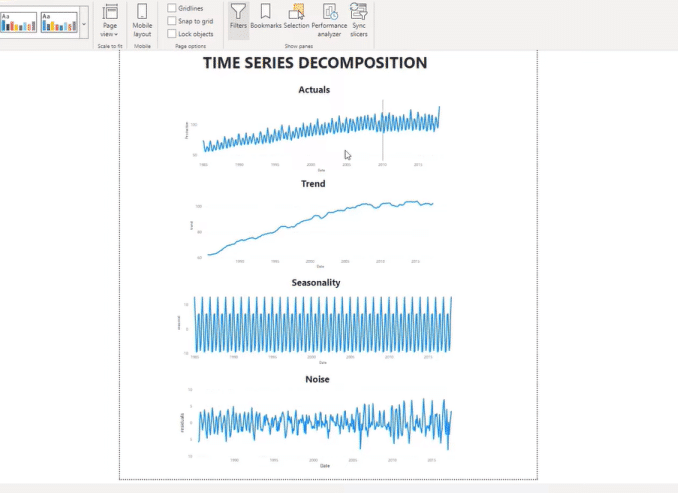
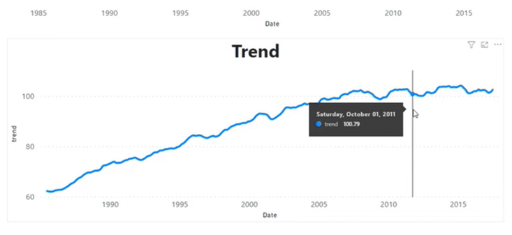
In the image above there are several graphs, including Actuals, Trends, Seasonality, and Noise. One of the best things about this visual is that there are dips in each graph.
This feature can come in handy when you want to highlight certain crucial factors that influence trends, like income and occupation in a consumer buying trend.
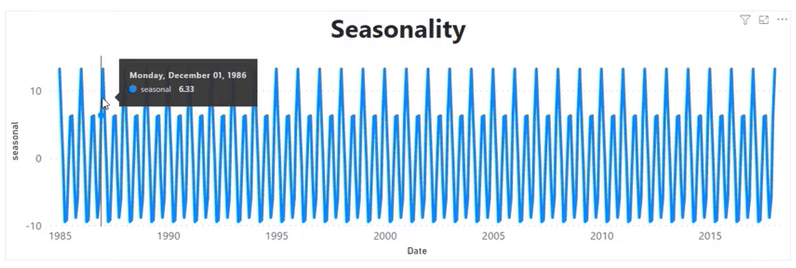
The same goes for pinpointing seasonal patterns, where they can describe a company’s monthly or quarterly growth movements.
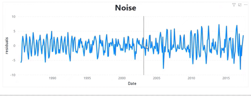
They are also excellent for determining data fluctuations like noise residual levels for scientific studies and the like. For example, we can see in the graph below an increase in residual levels for the last ten years, which gives us a bit of insight into a potential trend.
Understanding complex data movements throughout an extensive period are much easier when you present them through the above graphs. Digesting all the information and recognizing the patterns and trends in front of you is a lot easier.
As a result, that improves the interest and conversation surrounding your data report or presentation. It also helps you grasp what’s going on with your sales, production, or something else.

Power BI Time Series Data Set
I will show you two ways to break down this data series, which was created in Python Scrip Editor. I will also teach you how to create a Python visual using the same information. Finally, I will give you an idea of what you need to put into the Power Query.
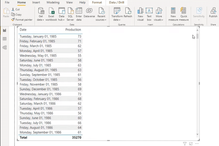
Below is our sample data set with a monthly date column from 1985 to 2018 alongside a production value column of a machine.
Python Script
Next, we’ll go to Python Script Editor and add a code to the two columns of our data set. The code will be importing pandas as pd, a data manipulation library, and matplotlib.pylot as plt, which shows our visuals. And for our seasonal decompose, it will be importing a package of statsmodels and tsa.seasonal.
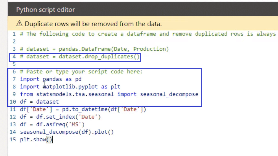
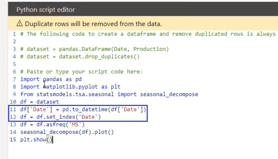
The variable in the 4th line shows where our data is saved, and in the 5th line, you’ll find that I changed our dataset name to df as it’s easier to write. And in the 11th line, I ensured that the date was set for date time and then made the index the date on the 12th.
Power BI Time Series Seasonal Decompose
To do a seasonal decompose, we need to have an index that’s a time series or a date time index. Thus, we’ll set the data index as the date and the first column.
We also want to set the frequency of the data into Month Start (MS) using the df variable alongside the freq function, as shown in the 13th line below.
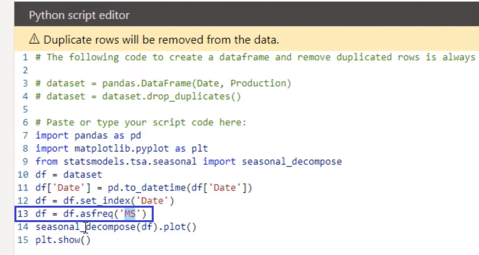
Finally, we use plt.show to see what we’ve created. And if we run that, we’ll have the result below.
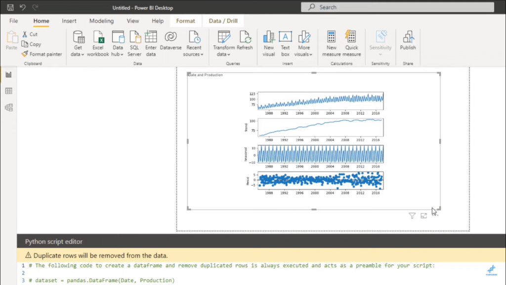
Now we have our seasonal decompose. And as you can see from the image above, it has our Actuals, Trend, Seasonality, and Residuals. These graphs will give you plenty of information on what’s going on with your sales or production over time.
Creating Visual with Power BI Time Series Data
Let’s go back to that main page so I can show you how I created these graphs within the data. Then we’ll go to Transform and see our original data set below, which is about Electric Production.
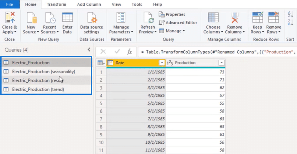
As you can see, I made three tables for Seasonality, Residuals, and Trends. It was hard to fit them together on one table, so I broke them into three. But it’s easy to copy and paste the code of our data.
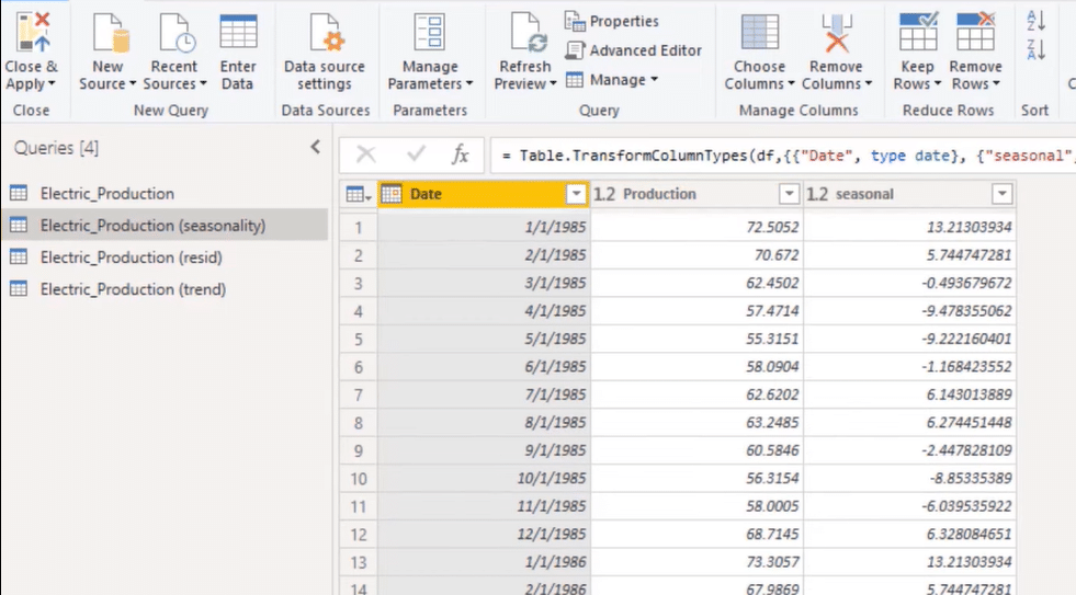
Seasonality
If we move to the Electric Production table, you will see that it has seasonality, date, and production columns. The seasonality column will show the fluctuation over time. We’ll go over the steps of creating it.
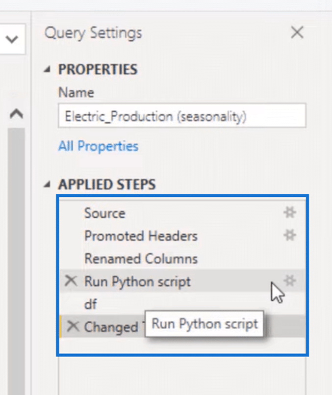
If we head over to the Applied Steps, you can see that I have already promoted the headers and renamed the columns, among others. What we’ll do here is click on the Run Python Script step.
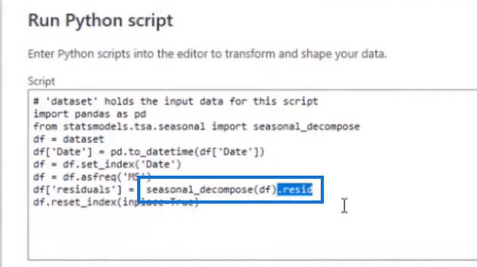
As you can see in the image below, we did almost the same thing we did for our visual when we created it in Python Visual. We’ve brought in our needed libraries, including pandas and statsmodels.tsa.seasonal and the seasonal_decompose function.
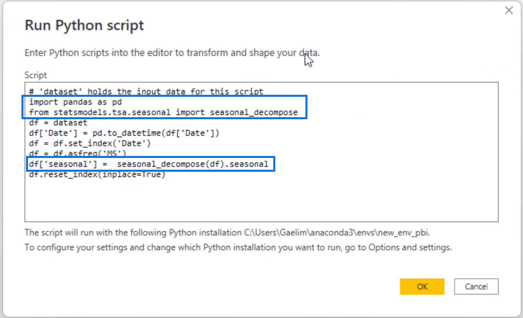
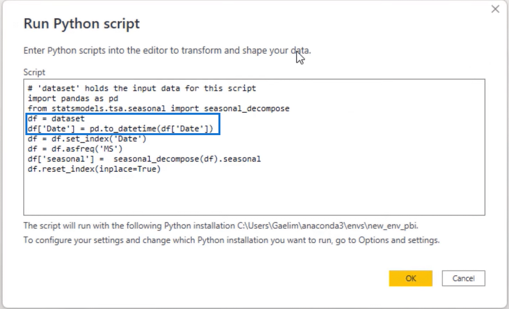
We also re-saved our data set variable as df for easier writing and created a date. To make sure that it was a date, we isolated the date column and then used pd.to_datetime. After that, we saved it over the df.
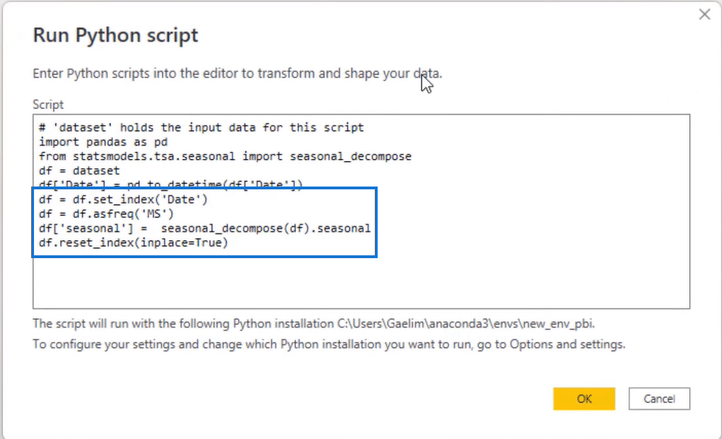
Then we changed the frequency to Month Start (MS) because we wanted to give those dates to the seasonal _decompose function.

Instead of plotting our function, we pulled out the seasonal part, passed in our data set, and used .seasonal just to bring out the seasonal data. Finally, we reset the index so we could see the date again.
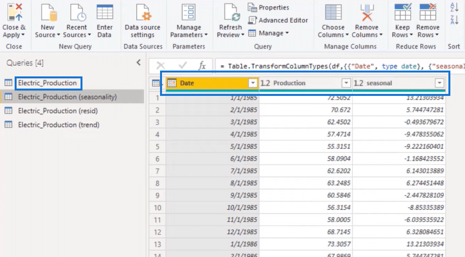
Now if I click OK, you can see that you are given the original data set and then the df that we stand for.
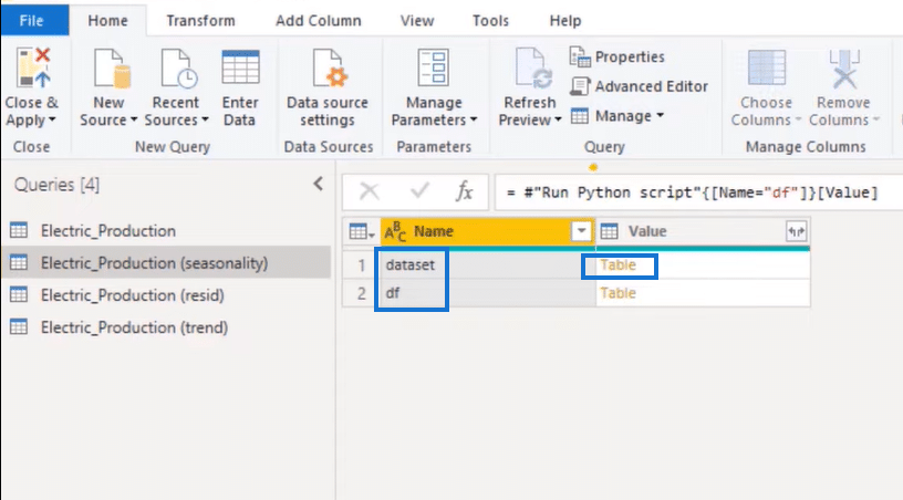
If we click on Table (highlighted in the image above) and open it, we’ll get the production seasonality table below. If you want to create a table similar to this one, just copy the script I showed you earlier.
Residuals
Now let’s move over to the Residuals where the only thing I’ve changed was the method or the point after the seasonal_decompose.
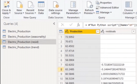
Not Resetting the Index
If we don’t reset the index and click OK, our script will return an error. So if we put a # before df.reset_index in the last line of our script, it will result in the table below. As you can see in the image, the index is missing and there’s no date column.
Thus, we need to reset the index because it returns the date, which would operate as this index. So if we remove that #, it will give me back the data frame, resulting in the table below, which now has a date column.
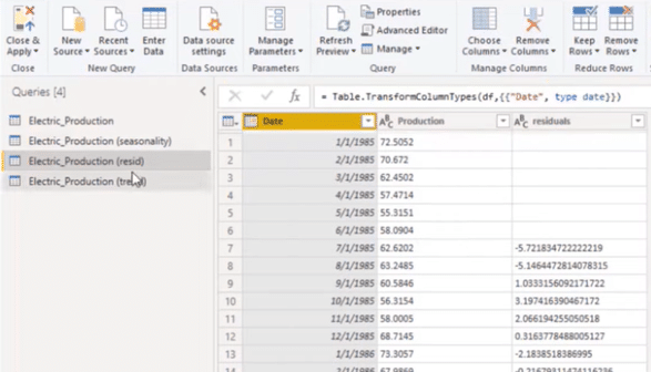
And you can use the same method for Trend, making it a really easy script that you can access anytime you want.
***** Related Links *****
Inventory Management Reports To Show Trends In Sales
Retail Management & Demand Forecasting Reports In Power BI
Power BI Data Visualization Tips For KPI Trends Analysis
Conclusion
Now you know a great way of breaking down your visuals. With a simple script, you can start creating Seasonality, Trend, and Residual time series data visuals in Power BI and Python.
With this Power BI time series decomposition method, you can describe data involving sales trends, seasonality growth and changes, or unexpected events. It’s also a great tool for forecasting. And the best part is you can easily copy and paste this script for any time series data you have.