There are times when you want to count the number of non-blank cells in a list in Excel and by excluding empty cells, you can get a more accurate picture of your data.
The most common method to count non-blank cells in Excel is to use the COUNTA function with the range of cells to be evaluated. Other methods include the COUNTIF function and the Find-And-Replace tool.
This article shows you how to count non-blank cells in Excel with five methods:
the COUNTA function
combining SUM and COUNTA
COUNTBLANK
COUNTIF
Find-And-Replace
You may not be familiar with some of these Excel formulas but our examples show exactly how to use them.
1. Using The COUNTA Function
The COUNTA function is a built-in Excel function that counts cells that are not empty. It provides the opposite results to the COUNTBLANK function.
It works on ranges that contain any type of data, including text, numbers, and formulas. The function accepts a list of up to 255 values. The list can be a range of cells.
This is the syntax: COUNTA(value1, [value2], …)
Let’s say you have a list of salespeople and their sales figures for the month:
[Create Table: Salesperson Sales John 10000 Jane Bob 5000 Sue 7500 Mike]
To count the number of salespeople who made a sale, type this formula into an empty cell and press enter:
=COUNTA(B2:B6)
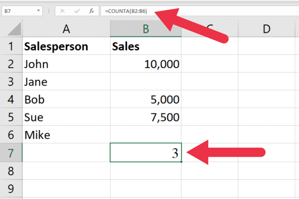
This formula counts the number of cells in the range B2:B6 that are not empty. In this case, the result would be 3, since only three salespeople made a sale.
The picture below shows an Excel spreadsheet with the function in the formula bar.
Why Not Use The COUNT Function to Count Non-Empty Cells?
If you’re familiar with the more commonly used COUNT function, you’ll probably know that we could use COUNT in the above example and get the same result (i.e. 3 filled cells).
The difference is that it will count cells that only include numerical values. It ignores text or logical values (TRUE or FALSE).
Suppose we replaced the sales numbers with text values like 10K, 5K, and 7.5K.
The COUNT function will return a zero, while the COUNTA function shows 3 non-blank cells.
How to Count Multiple Lists
You can also use the COUNTA function to count each non blank cell in more than one range.
For example, if you had another list of salespeople and their sales figures for a different month, you could use the following formula:
=COUNTA(B2:B6, D2:D6)
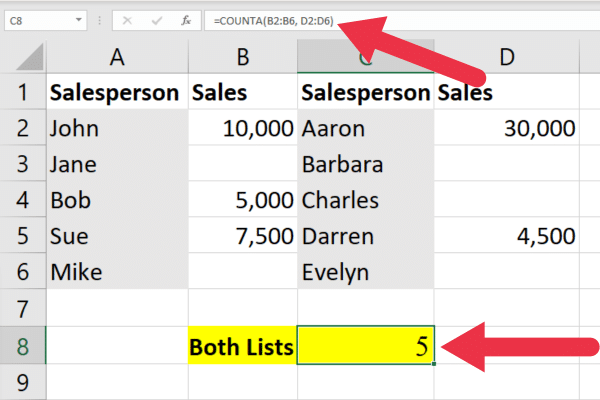
This formula counts the number of selected cells in the range B2:B6 and D2:D6 that are not empty.
In the case of the illustration, the result would be 5. That’s because five salespeople made a sale in either of the two months.
How to Count Distinct Values
After you count non empty cells in a large table, you may want to count the distinct values. This video will show you how:
2. How to Use SUM And COUNTA Together
You can also achieve the same results by combing the SUM function with the COUNTA function to count the number of non-blank cells in several ranges.
Using the data in the previous example, the formula looks like this:
=SUM(COUNTA(B2:B6), COUNTA(D2:D6))
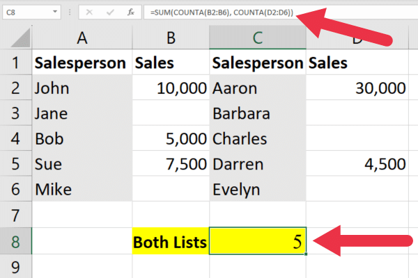
The COUNTA function is used to count the number of cells that are not blank in each of the two ranges, B2:B6 and D2:D6.
Then, the SUM function is used to add up the two counts to get the total count of non-blank cells in both ranges.
3. How to Use The COUNTIF Function
The COUNTIF function in Excel counts the number of data values in a range that meets a specific condition or criteria. It takes two arguments: the range of all the cells you want to count, and the criteria you want to apply.
This is the syntax: =COUNTIF(range, criteria)
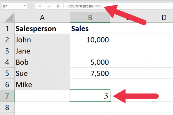
The criteria can include logical operators. Using our sample data, we can count the number of non-blank cells with this COUNTIF formula:
=COUNTIF(B2:B6,”<>”)
The first argument is the range. The second argument uses the <> operator to specify the “not equal to” condition. The two quotation marks with nothing in between specify an empty string.
4. How to Use The SUMPRODUCT Function
The SUMPRODUCT function is an array formula used to multiply two or more arrays of values and return the sum of their products.
An array refers to a list of values. The cell range that contains the first set of sales figures is one array. The array that contains the other set is a second array.
This is the syntax: =SUMPRODUCT(array1, [array2], [array3], …)
The SUMPRODUCT function can also be used to count non empty cells and blank formulas.
Example
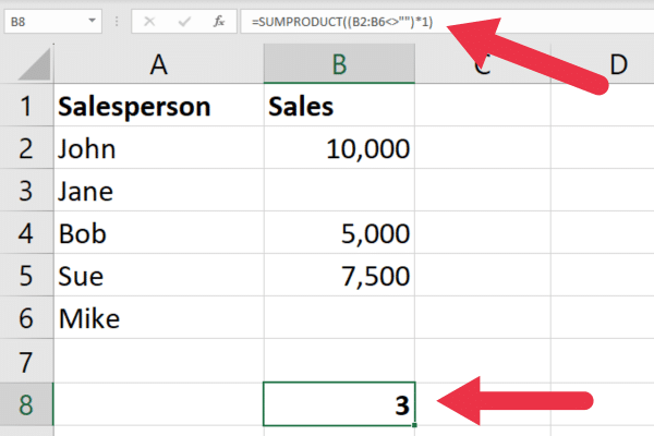
Taking our list of sales figures, we can count the non empty cells using this formula output:
=SUMPRODUCT((B2:B6<>””)*1)
The formula works by using the not equal operator to skip an empty cell in the range address.
5. How to Use Find And Replace
This method doesn’t use Excel formulas. Instead, you use the Find And Replace dialog box with these steps:
Select the column or range you want to check.
Open the Find And Replace dialog box (press ctrl + f ).
Enter the asterisk symbol in the “Find what” input box.
Click on the “Options” button to expand the dialog box and show more options.
Make sure the “Look in” field is set to “Values”
Check the “Match entire cell contents” option.
Click on the “Find All” button.
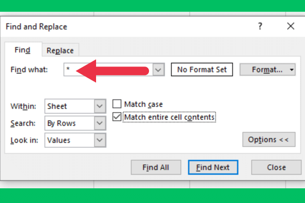
Excel will then display a list of all the non-blank cells in the selected range with their cell addresses. You can use this list to navigate to the non-blank cells or to select them all at once.
A Little Recap
In this article, we’ve given you 5 actionable ways how to count non-blank cells in Excel. Sure, there could be more, but we’ve found these methods to be the most useful an effective, and hope you do too!


