
Do you ever feel like your Excel data is playing hide-and-seek with you? It’s there, but sometimes it’s just not showing up in the right places.
One of the most common reasons for this is duplicate data, have no fear, we’ve got your back when it comes to finding and managing duplicates.
To count duplicates in Excel, you can use the COUNTIF function. It counts the number of occurrences of a value in a range. You can then filter and identify the values with a count greater than one, indicating that they are duplicates. functions.

Let us further explain.
Duplicate values can sneak into your data without you even realizing it. They can cause confusion and errors in your analysis. That’s why it’s important to have a good handle on finding and managing duplicates in Excel.
In this article, we’ll show you multiple methods to count duplicate values in Excel, making your data more accurate and easier to work with.
Time to dive in!

3 Ways to Calculate Duplicates in Excel
In this section, we’ll go over 3 different ways to find and manage duplicates in Excel. Each method has its own advantages and use cases, so you can choose the one that works best for you.
All methods are effective, but it comes down to personal preference, we’ll start with the COUNTIF function.

1. Using the COUNTIF Function
You can use the COUNTIF function to count duplicates in a range of cells. The syntax for the COUNTIF function is:
range: The range of cells in which you want to search for duplicates.
criteria: The value you want to count in the range.
For example, if you want to count the number of times the value “apple” appears in the range A1:A10, you can use the formula:
=COUNTIF($A$1:$A$10,A1)
In this case, the formula will count duplicate instances in the range A1:A10. You can then use this count to identify and manage the duplicates.
To identify duplicates, you can use the =COUNTIF(range, cell) function within an IF statement, like this:
=IF(COUNTIF($A$1:$A$10,A1)>1,”Duplicate”,”Unique”)
This formula checks if the count of the value in cell A2 is greater than 1. If it is, it returns “Duplicate,” otherwise, it returns “Unique.”
You can then copy this formula down to the other cells in the list to identify all the duplicates.
2. Using Conditional Formatting
Conditional formatting is a powerful feature in Excel that allows you to automatically format cells based on specific criteria.
You can use conditional formatting to identify and manage duplicate values in a range of cells.
To highlight duplicate values in a range of cells, you can follow these steps:
Step 1
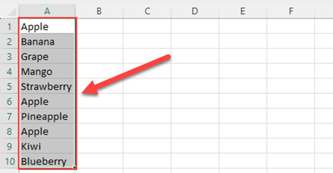
Select the data range that you want to check for duplicates.
Step 2
Go to the “Home” tab on the ribbon.

Step 3
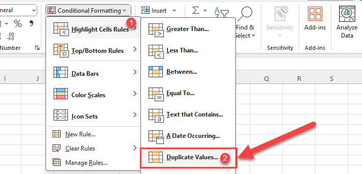
Click on “Conditional Formatting” in the Styles group.
Step 4
Choose “Highlight Cells Rules” and then “Duplicate Values” from the menu.
Step 5
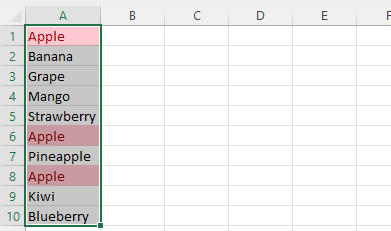
In the “Duplicate Values” dialog box, select the formatting options you want to apply to the duplicate values and click “OK.”

Excel will now highlight all the duplicate values in the selected range based on the criteria you specified.
You can use the above method to highlight duplicate rows also.
3. Using Advanced Filter
You can use the Advanced Filter feature in Excel to filter and extract duplicate values from a range of cells.
To do this, follow these steps:
Step 1
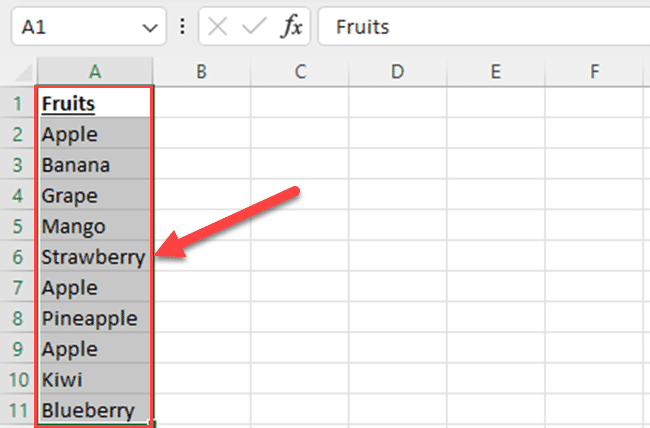
Select the range of cells that you want to filter.
Step 2
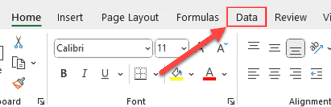
Go to the “Data” tab on the ribbon.
Step 3
In the “Sort & Filter” group, click on “Advanced.”
Step 4
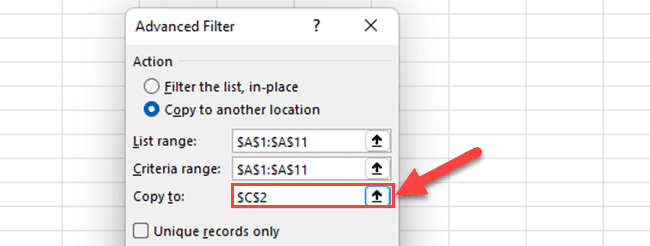
In the “Advanced Filter” dialog box, select “Copy to another location” as the action you want to perform.
Step 5
In the “List range” field, enter the range of cells that you want to filter.

Step 6
In the “Criteria range” field, enter the range of cells that contains the criteria for the filter. This should include the column header and the value you want to filter by.
Step 7
In the “Copy to” field, enter the reference for the cell where you want to copy the filtered data.
Step 8
Check the “Unique records only” checkbox to copy only the unique values to the specified location.
Step 9
Click “OK.”
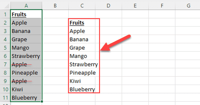
Excel will now copy the unique values from the specified range to the specified location, leaving out the duplicates.
How to Remove Duplicates in Excel
In this section, we’ll go over the steps to remove duplicates.
You’ve found them, now it’s time to remove these sneaky duplicates, luckily Excel provides a simple way to remove duplicates using built-in tools.
1. Removing Duplicates from a Single Column
To remove duplicates from a single column, follow these steps:
Select the range of cells that contains the column you want to check for duplicates.
Go to the “Data” tab on the Excel ribbon.
In the “Data Tools” group, click on “Remove Duplicates.”
In the “Remove Duplicates” dialog box, select the column(s) you want to check for duplicates and click “OK.”
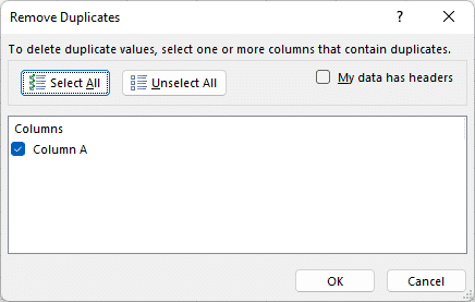
Excel will remove the duplicate values from the selected column and display a message with the number of duplicate values removed.
2. Removing Duplicates from Multiple Columns
To remove duplicates from multiple columns, follow the same steps as above, but in the “Remove Duplicates” dialog box, select the columns you want to check for duplicates.
Excel will remove the duplicate values from the selected columns and display a message with the number of duplicate values removed.
How to Handle Duplicate Data in Excel Tables
Duplicates can appear anywhere; in this section, we’ll specifically go over how to handle duplicate data in Excel tables.
1. Using Pivot Tables
Pivot tables are a powerful tool in Excel that allows you to summarize and analyze data from a table or range. You can use pivot tables to identify and handle duplicate data in a table.
To create a pivot table, follow these steps:
Select any cell in the table.
Go to the “Insert” tab on the ribbon.
In the “Tables” group, click on “PivotTable.”
In the “Create PivotTable” dialog box, select the range of cells you want to analyze and choose the location where you want to place the pivot table.
Click “OK.”
Excel will now create a pivot table in the specified location.
To analyze duplicate data, follow these steps:
In the “PivotTable Fields” pane, drag the column you want to analyze to the “Rows” area.
Drag the same column to the “Values” area.
In the “Values” area, click on the drop-down arrow next to the column name and select “Count.”
Excel will now display the count of each value in the specified column, allowing you to identify duplicate data.
If the count is greater than 1, that item has a duplicate value.
Wrap Up
We hope this article has given you a better understanding of how to calculate duplicates in your spreadsheets.
Whether you’re dealing with large datasets or just a few cells, managing duplicates is a crucial part of maintaining data integrity.
Remember that there are multiple methods to identify and handle duplicates, and the right approach depends on the specific requirements of your data and the tools you have at your disposal.
As you continue to work with Excel, you’ll find that these techniques will help you keep your data clean and make your analysis more accurate and efficient.
If you’re interested in a complete learning experience that covers AI, Excel, Power BI, and Python, check out our video below:
Frequently Asked Questions
In this section, you’ll find some frequently asked questions that you may have when calculating duplicates in Excel.
How do I count duplicates in Excel?
To count duplicates in Excel, you can use the COUNTIF function. This function counts the number of occurrences of a value in a range. For example, to count the number of times the value “apple” appears in the range A1:A10, you can use the formula =COUNTIF(A1:A10, “apple”).
How do I highlight duplicates in Excel?
To highlight duplicates in Excel, you can use conditional formatting. Select the range of cells you want to check for duplicates, then go to the “Home” tab, click on “Conditional Formatting,” and choose “Highlight Cells Rules” and then “Duplicate Values” from the menu. Select the formatting options you want to apply and click “OK.”
How do I identify duplicates in Excel?
To identify duplicates in Excel, you can use the COUNTIF function within an IF statement. For example, to identify duplicates in a list of values in column A, you can use the formula =IF(COUNTIF($A$1:A1, A1)>1, “Duplicate”, “Unique”). Copy this formula down to the other cells in the list to identify all the duplicates.
How do I delete duplicates in Excel?
To delete duplicates in Excel, you can use the “Remove Duplicates” feature. Select the range of cells you want to check for duplicates, then go to the “Data” tab, click on “Remove Duplicates,” and select the columns you want to check. Excel will remove the duplicate values from the selected columns and display a message with the number of duplicate values removed.
How do I find duplicates between two columns in Excel?
To find duplicates between two columns in Excel, you can use the COUNTIF function with an AND statement. For example, to find duplicates between columns A and B, you can use the formula =IF(AND(COUNTIF(A:A, A1)>1, COUNTIF(B:B, A1)>0), “Duplicate”, “Unique”). Copy this formula down to the other cells in column A to find all the duplicates.
How do I calculate duplicates in a pivot table?
To calculate duplicates in a pivot table, you can use the COUNTIF function in the “Values” area. Drag the column you want to analyze to the “Rows” area, then drag the same column to the “Values” area. In the “Values” area, click on the drop-down arrow next to the column name and select “Count.” Excel will display the count of each value in the specified column, allowing you to identify duplicates.


