
Having phone numbers correctly formatted in Excel makes for a clean and organized spreadsheet.
Luckily, it’s super easy to do.
To format phone numbers in Excel:

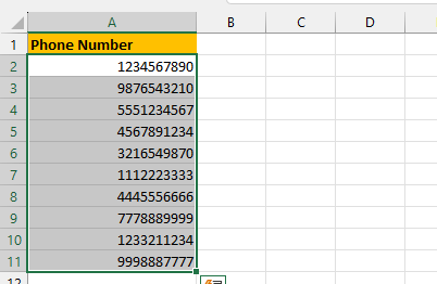
Select the cells with the phone numbers you want to format.
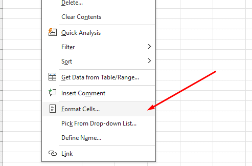
Right-click and choose the “Format Cells” option.
In the “Format Cells” dialog box, select the “Special” category.
Choose the “Phone Number” option.
But wait, there are more ways to go about this.
In this article, we’ll provide a step-by-step guide to help you properly format phone numbers in Excel.
We’ll also explore different formatting techniques and provide examples to make the process clear and easy to follow.
Let’s get started!
Basics of Formatting Phone Numbers in Excel

In this section, we’ll review the best, most straightforward methods for formatting phone numbers in Excel using the Format Cells dialog box and a custom format.
1. Format Cells Dialog Box with a Custom Format
The Format Cells dialog box is an essential tool for adjusting the appearance of data in your Excel spreadsheets. It allows you to apply various formatting options, including changing the number format.

Follow the steps below to format phone numbers in Excel using a custom format:
- Select the cells containing the phone numbers you want to format.
- Right-click the selected cells and choose Format Cells from the context menu.
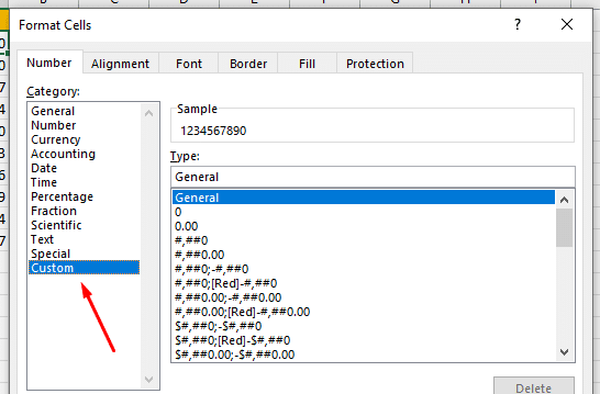
- Select the Number tab in the Format Cells dialog box, and then choose Custom from the Category list.
- In the Type field, enter a custom format code for the phone numbers. For example, use “(###) ###-####” to format a 10-digit U.S. phone number.
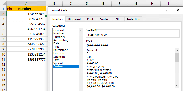
- Click OK to apply the format.
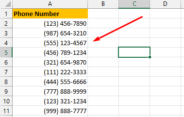
This process will change the appearance of the selected cells to display phone numbers in a standardized format, such as (123) 456-7890.
Next up, let’s take a look at using the text function to handle format phone number formats.
2. Using the Text Function
Another way to format phone numbers in Excel is by using the TEXT function. This function allows you to convert a numeric value to text in a specific format.
The syntax of the TEXT function for formatting phone numbers is:
TEXT(value, format_text)value: This is the cell reference or numeric value that you want to format.
format_text: This is a text string that defines the desired format.
Let’s take a look at an example.

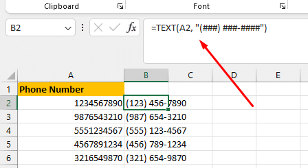
Suppose you have a list of phone numbers in the column A, and you want to format them in the (###) ###-#### format. You can use the following formula:
In this formula:
A2 is the reference to the cell containing the phone number.
“(###) ###-####” is the format you want to apply.
After applying the formula, the phone number will be displayed in the desired format.
You can format phone numbers in Excel using the Format Cells dialog box or the TEXT function. The Format Cells method is more straightforward, while the TEXT function provides more flexibility in customizing the format.
3. Advanced Formatting With Conditional Formatting
Conditional formatting is a powerful feature in Excel that allows you to apply specific formatting to cells based on certain conditions.
You can use conditional formatting to format phone numbers based on their values automatically.
For example, you can apply different formats to phone numbers based on their length or the area code.
Follow the steps below to apply conditional formatting to format phone numbers based on their length:
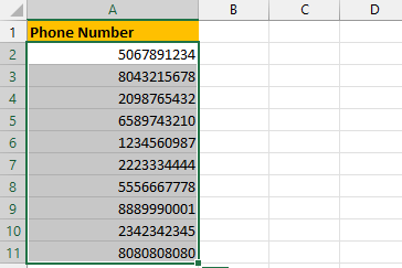
- Select the cells containing the phone numbers you want to format.
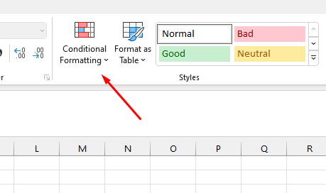
- Go to the Home tab on the ribbon.
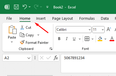
- Click on the Conditional Formatting option in the Styles group.
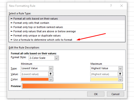
- Choose New Rule from the drop-down menu.

- In the New Formatting Rule dialog box, select the Use a formula to determine which cells to format option.
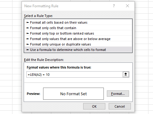
- Enter the following formula: =LEN(A2) = 10. Replace A2 with the first cell reference in your selected range.
- Click on the Format button and choose the desired formatting for the phone numbers that meet the condition.
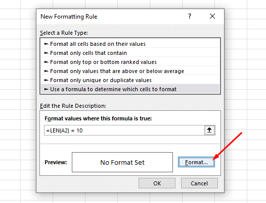
- Click OK to apply the conditional formatting to your numbers.
In this example, we applied conditional formatting to format phone numbers with 10 digits. You can adjust the formula and formatting to meet your specific needs.

Final Thoughts
Mastering the art of formatting phone numbers in Excel can significantly enhance your data management skills.
Whether you’re a seasoned spreadsheet aficionado or a novice just dipping your toes into the world of data manipulation, the ability to present phone numbers in a clear, consistent manner is invaluable.
By applying the techniques we’ve discussed, you can ensure that your phone numbers are not only neatly arranged but also easily recognizable. This can be especially useful when dealing with large datasets or when sharing information with others.
Lastly, understanding the different methods of formatting phone numbers in Excel can help you find what works best for your skills and use case.
Wanna learn more about About awesome Excel features like Tracking changes using dimensions in Power Query?
Checkout this great video on our YouTube channel:
Frequently Asked Questions
How do I change the phone number format in Excel?
To change the phone number format in Excel, you can use the “Format Cells” option. First, select the cells containing the phone numbers you want to format. Then, right-click and choose “Format Cells.” In the “Format Cells” dialog box, select the “Special” category, and choose the “Phone Number” option.
How do I format a cell to show the phone number in a particular way?
To format a cell to show the phone number in a particular way, you can use the “Custom” category in the “Format Cells” dialog box.
Right-click on the cell you want to format, choose “Format Cells”, and then select the “Custom” category. In the “Type” field, enter the desired phone number format using pound signs (#) for digits and other characters as needed.
What is the best format for phone numbers in Excel?
The best format for phone numbers in Excel is the one that suits your needs and preferences.
Common formats include (###) ###-#### for US numbers and +CC NDC XXX XXXX for international numbers, where CC is the country code and NDC is the national destination code.
How to remove formatting from phone numbers in Excel?
To remove formatting from phone numbers in Excel, you can use the “Clear” option. First, select the cells with the formatted phone numbers.
Then, right-click and choose “Clear” from the context menu. In the “Clear” dialog box, select the “Formats” option and click “OK.”
How to format phone numbers with an extension in Excel?
To format phone numbers with an extension in Excel, you can use a custom number format. Select the cells with the phone numbers and apply the following custom format: “(000) 000-0000####.” Replace the pound signs with the appropriate digits for the extension.
How to convert phone numbers to text in Excel?
To convert phone numbers to text in Excel, you can use the “TEXT” function. For example, if the phone number is in cell A1, you can use the formula =TEXT(A1, “(000) 000-0000”) to display the number as text in the specified format.


