A game-changing feature of Microsoft Excel is the ability to quickly and accurately apply the calculation style.
To apply calculation styles in Excel:
Select the cells with calculations
Navigate to the Home tab
In the Styles section, you can choose conditional formatting, Format as Table, and Cell Styles options. Choose your desired option to highlight these cells.
This feature visually distinguishes cells, making them stand out for easier identification and analysis.
In this article, we’ll dig into the specifics of the Calculation style option, helping you understand the 3 types of styles and how to use them effectively.
Let’s get Excelling!
3 Types of Styles in Excel
In this section, we will go over the 3 types of styles Excel offers, including:
Conditional Formatting
Format as Table
Cell Styles
1. How to Apply Calculation Style With Conditional Formatting
Conditional Formatting is a feature that allows you to apply specific formatting to cells that meet certain criteria. It’s incredibly useful for highlighting trends, exceptions, and key metrics within your data automatically.
To apply the calculation style with conditional formatting, follow the steps given below:
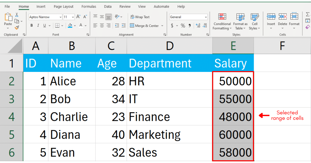
Step 1: Select Your Data
Highlight the cells or range in your worksheet where you want to apply conditional formatting.
Step 2: Access Conditional Formatting
Go to the Home tab on the ribbon, find the Styles group, and click on Conditional Formatting.
Select from the various rules available, such as highlighting cell rules, top/bottom rules, or using formulas to determine which cells to format.
In our case, we will use Color Scales.
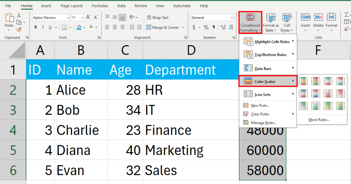
When you click a color scale of your choice, Excel will automatically style the cells in your selected range.
2. How to Apply Calculation Style With Format as Table
Format as Table allows you to quickly style your data range as a table with a consistent format and the ability to easily sort, filter, and manage your data.
To style cells or a range of cells using this method, follow the steps below:
Step 1: Select Your Data
Click on any cell within your data range.
Step 2: Format as Table
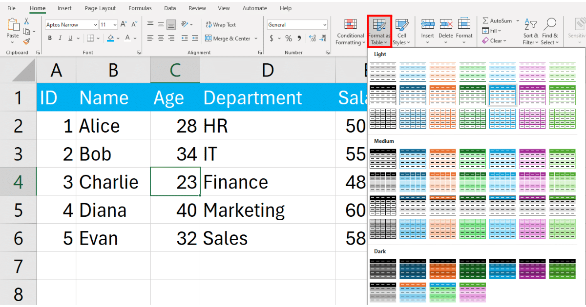
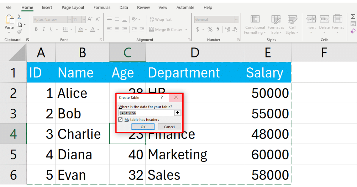
On the Home tab, in the Styles group, click Format as Table. Choose a table style from the dropdown menu.

Step 3: Table Options
Excel will automatically detect the data range for your table. Confirm the range and specify if your table has headers. Click ‘OK’ to apply the table format.
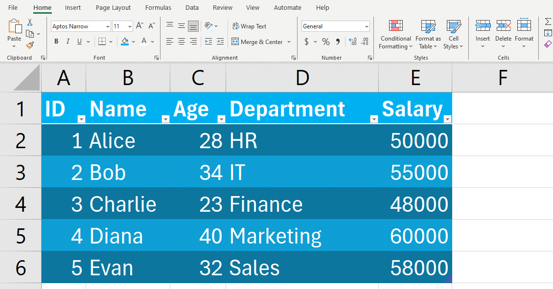
Excel will style the selected cells for you.
3. How to Apply The Calculation Style With Cell Styles
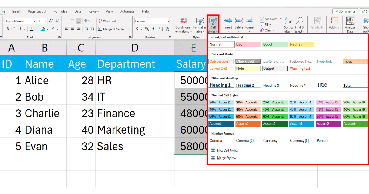
Cell Styles offers a collection of predefined styles that you can apply to improve the readability and appearance of your data.
Follow the steps given below to apply the calculation style with the cell style menu:
Step 1: Select Cells
Highlight the cells or range to which you want to apply a style.

Step 2: Apply Cell Style
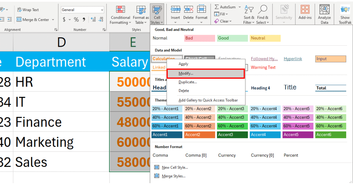
Go to the Home tab, click on Cell Styles in the cell styles menu, and choose from the variety of available styles.

Step 3: Customization
Select a style to apply it directly.
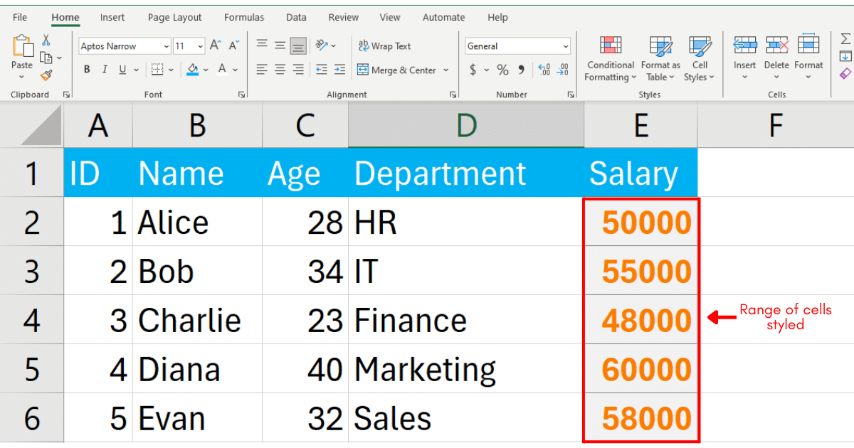
For more control, right-click on a style and choose ‘Modify’ to customize the style according to your needs.

When you click modify, a cell style dialog box opens up where you can customize the current calculation cell style.

Click OK to apply the changes.
With the cell style feature, you can make new styles, edit existing ones, and merge different styles as well.
Learn how you can supercharge your analytics journey with Enterprise DNA by watching the following video:
Final Thoughts
Utilizing the calculation style in Excel can greatly enhance the visual appeal, readability, and organization of your data.
After following the step-by-step guide provided, you can confidently apply this style to your cells with ease.
Lastly, by mastering the art of applying styles in Excel, you can create a professional showcase of your data that is easy to read and understand.
Frequently Asked Questions
In this section, you will find some frequently asked questions you may have when applying calculation style in Excel.

How can I apply a calculation style to a range of cells in Excel?
To apply a calculation style to a range of cells in Excel, first, select the desired range of cells. Then, go to the Home tab, click on the Styles group, and select the desired calculation style from the Cell Styles dialogue box.
The calculation style will be applied to the selected range of cells.
What are some common cell styles available in Excel?
Some common cell styles available in Excel include Normal, Currency, Comma, Percent, Title, Heading 1, and Total.
These styles can be accessed from the Cell Styles gallery in the Styles group of the Home tab.
How can I modify or create custom cell styles in Excel?
To modify or create custom cell styles in Excel, first, select the desired cell or range of cells. Then, go to the Cell Styles dialog box from the new Cell Style gallery on the Home tab and click on the Format as Table for Editing button.
In the Format Cells dialog box, you can modify the font, number format, alignment, border, and fill options to create a custom cell style.
How to apply Calculation styles?
First, you need to invest in converting all the plain text strings into factors that will automatically enable the Calculation cell style.
To apply the calculation style, first select the desired range of cells. Then, go to the Home tab, click on the Styles group, click the Cell Styles button, and choose the Calculation style from the list.
This style will display the cell content as plain text factor strings in italicized font with a blue border around the cells.
What is the Calculation style and when should it be used?
The Calculation cell style in Excel is a built-in style used to display cell content that is meant for calculation and not meant to be included in the final results.
This style is useful when working with data where some cells contain formulas or values that are for calculation purposes.


