I want to spend some time today talking about tables in Power BI. We run into tables all the time with every problem, but we don’t really spend a lot of time thinking about them alone. You can watch the full video of this tutorial at the bottom of this blog.
There was a post recently from Enterprise DNA member, Ashton, who always comes up with good, thought-provoking questions. His query got me thinking about a pattern that I see pretty regularly and want to address in this tutorial.
It wasn’t a mistake he made, but it’s a common mistake. I see many times where people would say they’re having trouble with a virtual table, for example, when it’s not a virtual table in the first place.
There’s a real distinction between the types of tables in Power BI.
The analogy I would give is if somebody said, “Hey, I’ve recently adopted a dog and I’m having trouble with the dog and wonder if you can help” and it’s not a dog, but a wolf. They’re both canines, but there are some pretty big distinctions that you want to take into account.
So while they’re all kind of the same family, just like the tables in Power BI, they are important distinctions that really affect the solution and how you use those tables. And so what I wanted to do was revisit Ashton’s question, and then delve a bit into the differences between the tables you find in Power BI and show how that influences the way you handle them.
The question was pretty simple, but there’s a little more to it than there initially appears. He had a simple data set that just says clients, the type of fruit they purchased, the quantity, and then just an index number.
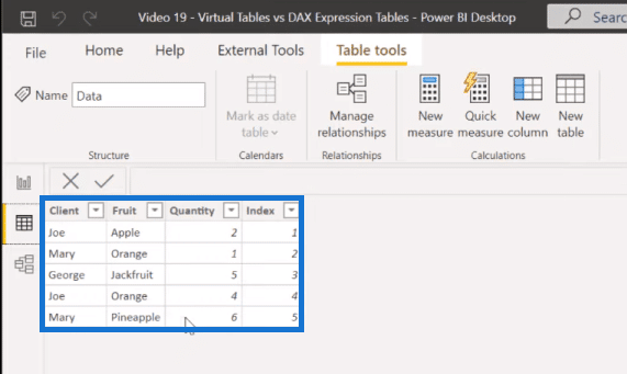
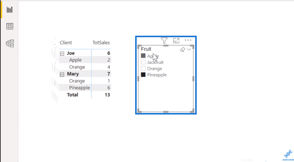
He wanted to have a slicer with a multi-select capability so that if you selected say orange, it would pull up all the clients who bought oranges, but it would also show what else they purchased.
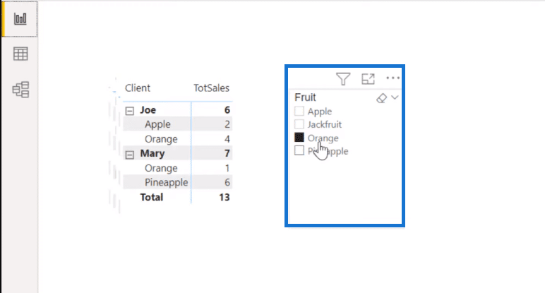
So, if we turn this selection (orange) off, we can see the full data set. We can also see that these are the two clients (Joe and Mary) who purchased oranges, but they each also had an additional purchase.
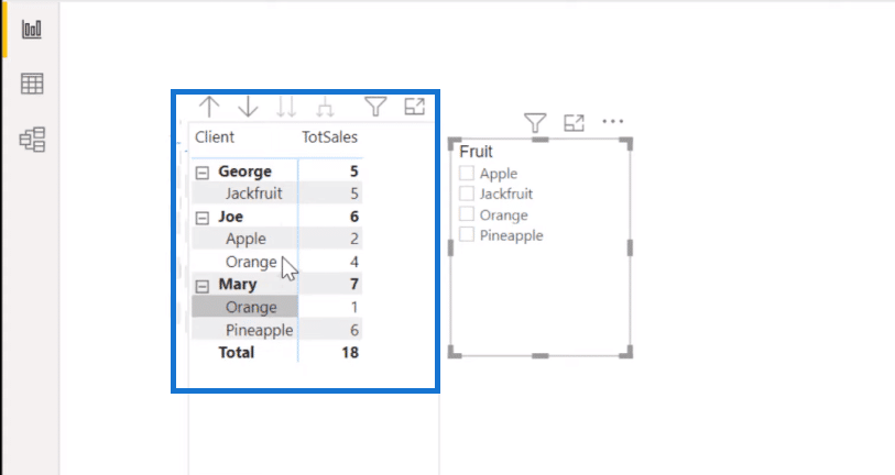
And so, the first thing we know about is that the Fruit slicer has got to be a disconnected slicer table. If it were a regular slicer, you’d hit orange and it would basically take out everything but orange in the table. We also know, because this is dynamic, we’ve got a virtual table issue.
So let’s delve into this a bit, but before we do, let’s take a look at the different types of tables that we find in Power BI.
Three Type Of Tables In Power BI
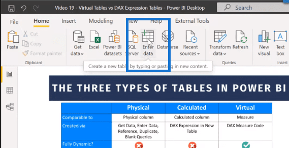
There are three types of tables that we find regularly. The first one is the most common and it’s a physical table, and this is really your primary data. Whenever you do Get Data or you Enter Data directly through this option or in Power Query, you do a Reference or Duplicate, or you load data through a Blank Query, like a Date table, that’s a physical table.
A physical table is not fully dynamic, but it does have all these other characteristics that increase file size because it is physical data. It’s accessible in Power Query. Typically the relationships in the data model are built through physical relationships. They don’t have to be, but they usually are. They’re used for primary data and you visualize it through either the data view or through Power Query.

A physical table is not fully dynamic, but it does have all these other characteristics that increase file size because it is physical data. It’s accessible in Power Query. Typically the relationships in the data model are built through physical relationships. They don’t have to be, but they usually are. They’re used for primary data and you visualize it through either the data view or through Power Query.
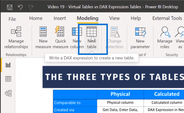
The one that often gets confused with the virtual table is this calculated table or what we can also refer to as a DAX expression table. This has a direct analogy to calculated columns that are created through DAX expressions. This is done through the Modeling tab and the New table option, and then you enter the DAX expression.
The one that often gets confused with the virtual table is this calculated table or what we can also refer to as a DAX expression table. This has a direct analogy to calculated columns that are created through DAX expressions. This is done through the Modeling tab and the New table option, and then you enter the DAX expression.
As you can see from the comparison table below, the calculated table is quite different in profile from either the physical table or the virtual table. It’s not fully dynamic.
It needs to be refreshed in order to pick up the new information. It does increase physical file size. Unlike a straight-up physical table, it’s not accessible in Power Query. Just like a calculated column doesn’t show up in Power Query, a calculated table doesn’t either. But it does possess the other aspects of a physical table.
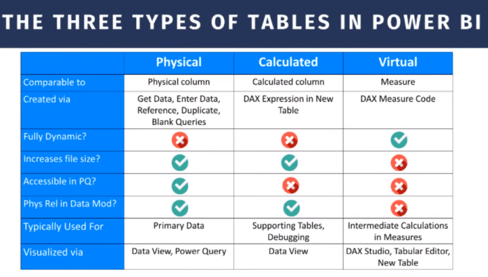
Typically, calculated tables used for supporting tables and used more commonly for debugging. There are now better tools like DAX Studio and Tabular Editor, so it’s not used as frequently for that. You view this table through the data view.
And frankly, like calculated columns, it’s generally something to stay away from. There are better ways of doing things than through calculated tables.
And then the analogy to measures are the true virtual tables. These are created in the context of measures through the DAX Measure Code. They are fully dynamic, unlike the other two types of tables. They don’t increase file size because they’re on-demand. Just like measures, virtual tables are calculated on-demand in memory and are all used over the course of contexts that they’re needed for.
They’re not accessible in Power Query. You can’t put a physical relationship on those. If you relate them in your data model, you do so using virtual relationships, most commonly with TREATAS.
Virtual tables are used for intermediate calculations in measures because a measure can’t return a table value and it has to return a scalar value. So you typically use those as the interim calculation upon which you generate your scalers, which are the resulting product of your measure.
You can visualize these tables in tools like DAX Studio, Tabular Editor, or New Table, which is again, probably the least desirable way because it clutters up your data model with a bunch of extra tables, unless you delete this.
DAX Measure Solution For A Virtual Table
Going back to Ashton’s question, by looking at the table, we can tell that it is dynamic. We can also do multiple choices and this changes fully on the fly. And so because of that, we know that it’s a virtual table because the other two (physical and calculated tables) are not fully dynamic. We also know that it’s a disconnected table, as I mentioned in the beginning.
I used the Rubber Duck concept to solve this. In a previous tutorial, I’ve talked about this concept of rubber ducking, which is developing a conceptual solution to the problem before you start digging into the specific DAX.
And so, for the rubber duck solution here, what I did was basically put together this disconnected slicer table. Then, I harvested the value of those slicers. Next, I came up with a virtual table that filtered clients by those who had purchased the selections in the disconnected table.
Then, I took that client list and filtered our original data set by those clients to come up with the clients and the purchases made by those clients, in addition to the slicer value.
Let’s take a look at the specific measure to see how this played out and some of the considerations you have in working with virtual tables.
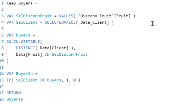
The first thing was to develop two harvest measures for our values. The first one being the value of the disconnected slicer.
Since we had the multi-select in the requirement, it meant we couldn’t just use SELECTEDVALUE. So what I did is use the VALUES function to capture potentially one or more selections in that disconnected slicer. For clients, since we’re going to have one client on each row that we’re evaluating, we can use SELECTEDVALUE.
The next thing I did was this virtual table variable (VAR Buyers) that starts with CALCULATETABLE. Then, it goes into filtering the DISTINCT clients by whether or not they made a fruit purchase that was in our values of the disconnected slicer.
We can check this out by doing a DAX query. We can do that in either DAX Studio or in Tabular Editor. So let’s take our virtual table measure here, copy it over into Tabular Editor. We’ll make sure that it’s giving us the values that we expect to see, which would be Joe and Mary.
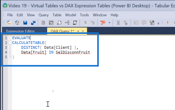
DAX queries always return tables and they always started with EVALUATE, so we add EVALUATE here. However, we’re not getting anything in the result. This is because the selected disconnect fruit (SelDisconnFruit) harvest variable has no awareness of the slicer. It’s out of context.
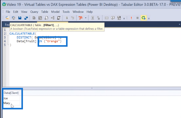
So the way to test that is kind of artificially setting that slicer value. We’ll replace SelDisconnFruit with a small table here. Type in Orange (the value of that slicer) between squiggly brackets. And now, we get the result here, which is Joe and Mary. With that, the virtual table is working just exactly as we thought it would.
So we can go back now to our measure expression. One of the challenging things about virtual tables is that they’re easy to create virtual tables within a measure. But you can’t return a virtual table as the result of a measure. So we need to return a scalar, but that captures the relevant aspect of the virtual table.
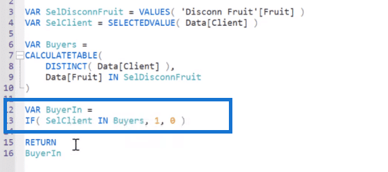
So here, we have the virtual table that tells us which clients purchased the fruits that were in the value slicer. We can set up another variable (VAR BuyerIn) that says, if the selected client was in that buyer’s table, then it gets a one. And if not, it gets a zero.
Then we take the results of that and put that into the filter pane. The Key Buyers measure, we say, is one and that’s going to be the clients that purchased, in this case, oranges.
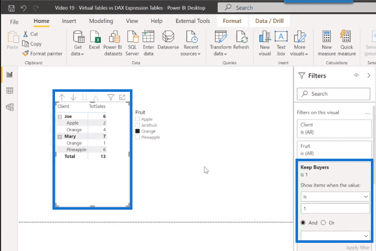
And so by doing that, we filter our original data table down to the correct records. You can see that it now creates that virtual table and it does that filtering properly based on each selection.
***** Related Links *****
Virtual Tables Inside Iterating Functions In Power BI – DAX Concepts
Creating Virtual Relationships In Power BI Using The TREATAS Function
How To Use The COUNTROWS DAX Function In Virtual Tables
Conclusion
That’s the bulk of what I wanted to cover today. It’s a fairly straightforward virtual table example, but with the focus on the difference between physical tables, calculated tables, and virtual tables.
There’s a lot of interesting issues to revisit with regard to virtual tables, particularly with debugging virtual table measures. That’s something I’ll be coming back to within the next few weeks, but for now, that’s all of this tutorial.
Cheers!
Brian

