Power BI Column Split Power Query Tutorial: How To Split Multi-Lined Excel Cells In Power BI

Table of Contents

Power Platform Tutorials

In this power query tutorial, I want to show you one way of splitting multiline cells into multiple rows. Sometimes you will get an Excel file where data inside the cell is split across multiple lines. Today, I want to show you how you can use Text.Split and List.Zip to help you out in a case like this. You can watch the full video of this tutorial at the bottom of this blog.

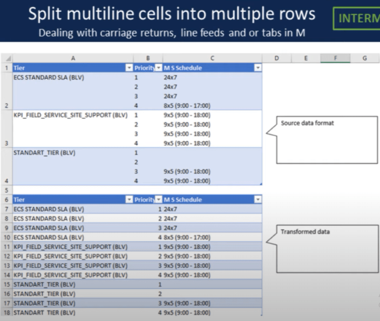
Let’s go over to power query.

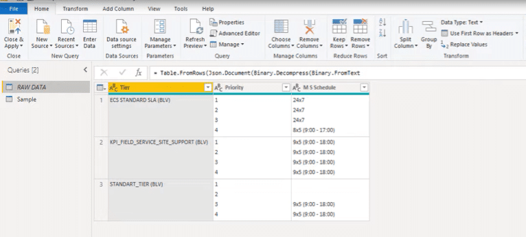
Before we do anything, make sure to have that formula bar visible on your screen. If it’s not visible, go to the View tab and toggle it on.

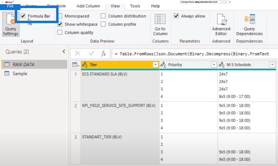
Second, let’s also find out how we can look for carriage returns or line feeds. For this one, I’ll open the advanced editor window and click on the question mark in the upper right corner.

This brings me straight to the online documentation. I’ll select the Power Query M language specification and go to Consolidated Grammar.

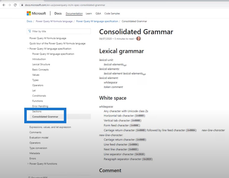
Let’s scroll down a bit to see Character escape sequences. This shows us how to write those carriage returns or line feeds. We need to start with a hash or a pound sign, followed by an opening parentheses and then the control character.

As you can see, those are two or three letters. It’s CR for carriage return, LF for line feed, or tab for tab, and then a closing parentheses.

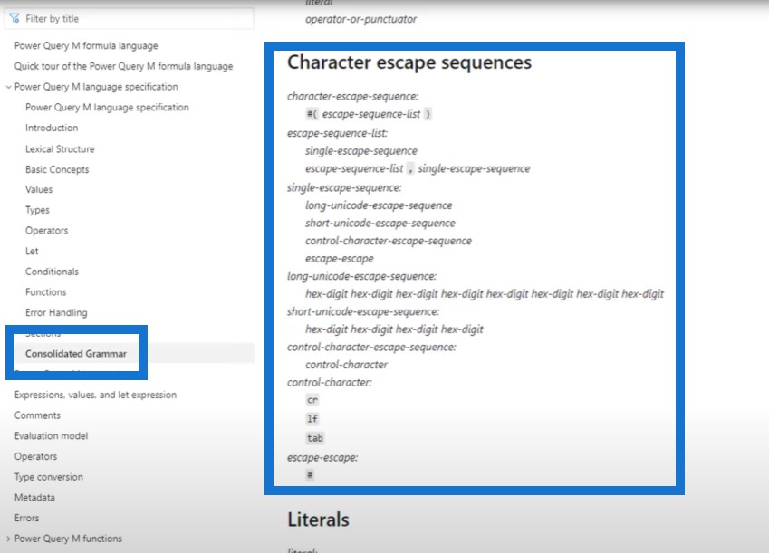
Splitting The Cells Into Multiple List Items

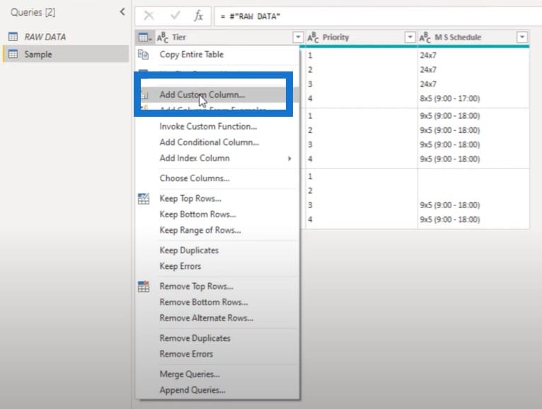
Let’s go back to our example, and discuss which one to use. We’ll add a custom column by clicking on the mini table icon in the top left corner and selecting Add Custom Column.

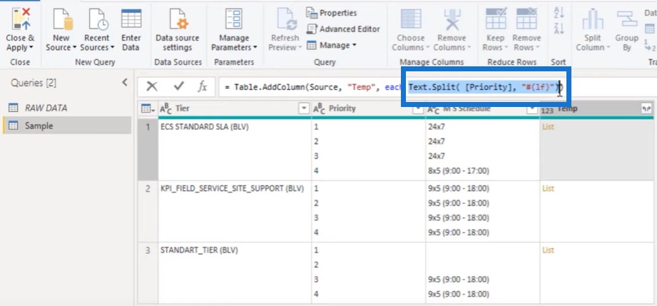
We’ll call this column Temp and enter a function called Text.Split.

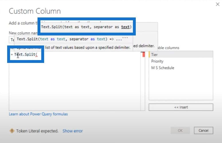
This function wants a text as a text and a separator as a text as well. So I’ll select Priority column, enter a carriage return, then press OK.

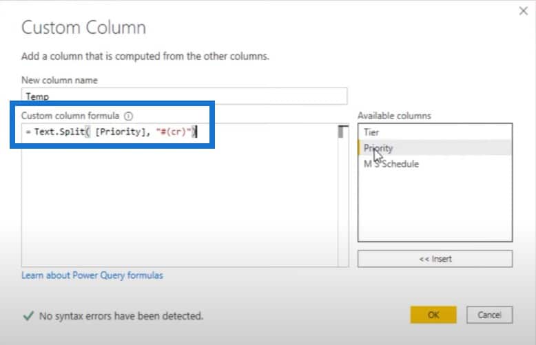
We’ll get a list as a result. When we click off to the side in the white space, we see a preview down below.

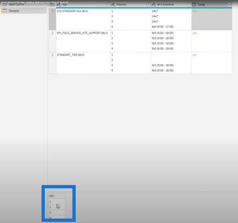
This is now working fine, so let’s go to our second column. We’ll click on the gear wheel icon and instead of Priority, let’s click on the M S Schedule column, then click OK.

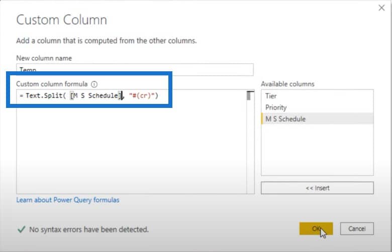
Let’s see the content. This is not looking good, so we’ll need to change this.

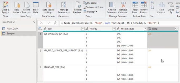
Let’s change something inside the formula bar. Let’s replace cr with lf (line feed), then press OK. Then click off to the side in the white space.

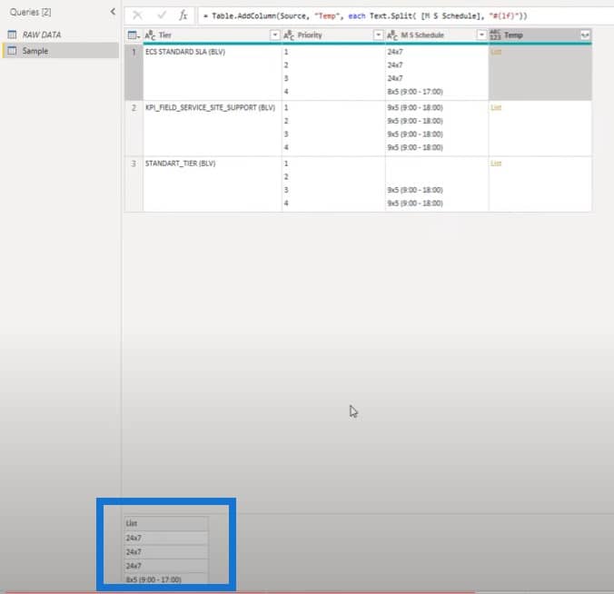
Let’s check this for our Priority column as well. We need the line feed for this one.

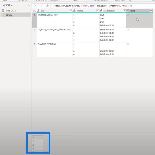
Bringing The Items Together Based On Position

Now that we know how to split our cells into multiple list items, we can bring the items together based on their position in that list to create a set of value pairs.

For that, we can use List.Zip. We’ll copy this section of the formula.

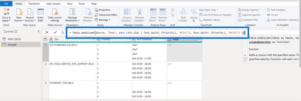
Then we’ll add List.Zip, opening parentheses, and then curly brackets to create a list containing lists. We’ll type in a comma, then paste in that piece of code again, and then the closing curly bracket and closing parentheses.

Let’s also change the column reference here from Priority to M S Schedule, and press OK.

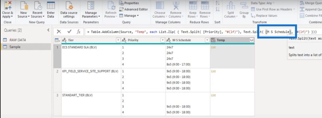
Click off to the side in the white space, and you can now see a list containing multiple lists.

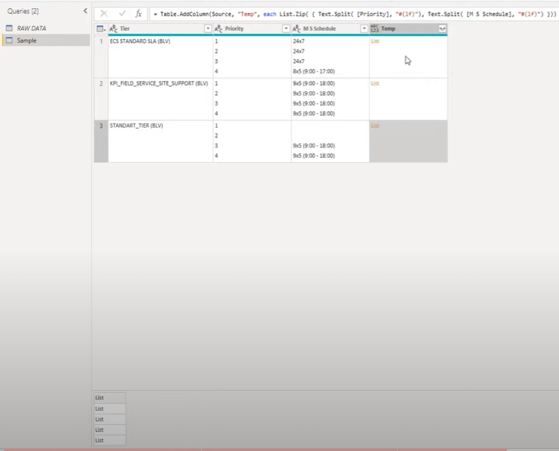
Let’s add one as a new query so we can see the contents, because we need to get those value pairs together.

Keeping Selected Columns

We can also keep only the columns that we want. We’re only interested in the first column that’s called Tier and in the column that we just created called Temp.

In a set of square brackets, we can point to the columns that we want to keep. Those column names need to pass in a set of square brackets as well.

So let’s type in the square brackets, then Tier, which is our first column. We’ll type in comma, then another set of square brackets and Temp.

We’re left with this small table, which we can expand to new rows.

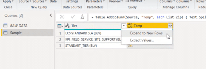
When we click on the left icon, we can see the option to extract the values.

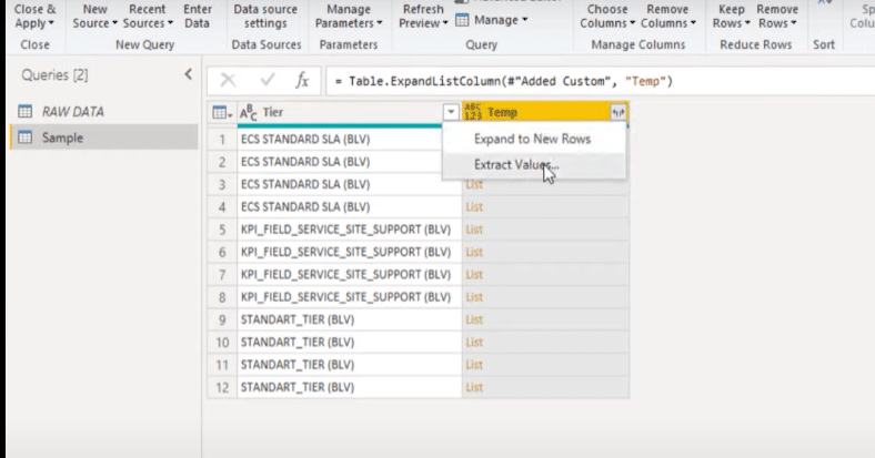
Let’s add a custom delimiter, then press OK.

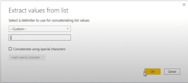
Well, we’re not quite there yet and we need to do some cleaning up.

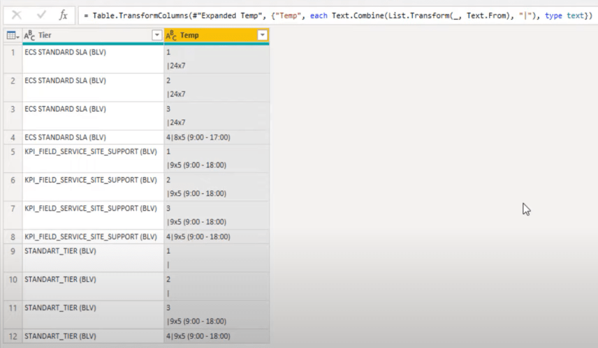
So let’s go to our Add custom column step.

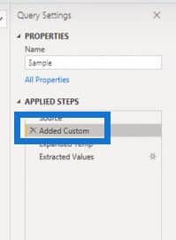
We need to transform the contents of this list.

We need to use a function called List.Transform, so I’ll add that here in the formula bar.

We also need to clean up those texts using the Text.Clean function.

Let’s head back to the final step. The results are awesome.

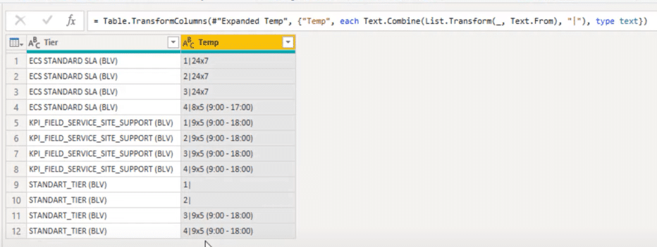
Splitting Column By Delimiter

Well, all that’s left to do is split the right column by the delimiter that we’ve given it.

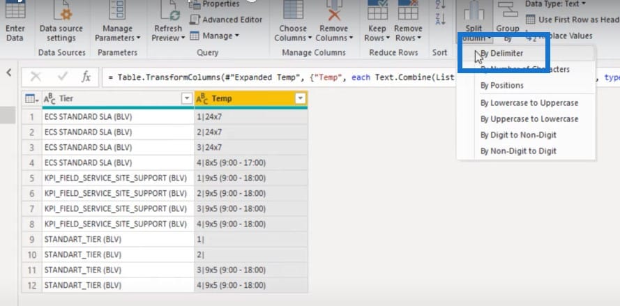
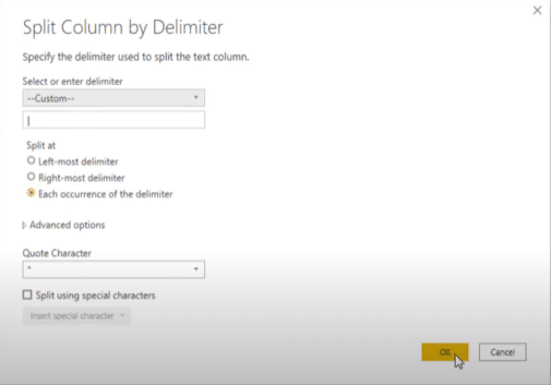
Lastly, inside the formula bar, we can give those columns back their proper names. The first one was called Priority and the second one was M S Schedule.

Conclusion

To summarize this power query tutorial, we’ve used character escape sequences to look for line feeds and carriage returns. We also learned how to use them to split multiline cells into multiple rows to turn our data back into a proper tabular format.

That’s all for now, and if you’ve enjoyed the content covered in this particular tutorial, please subscribe to the Enterprise DNA TV channel. We always have a huge amount of content coming out all the time dedicated to improving the way that you use Power BI and the Power Platform.

Melissa