
As a data scientist working with Python, you’ve most likely come across the NumPy library. It’s one of the foundational packages for scientific computing in Python.
With its ability to perform high-performance operations on multidimensional arrays, NumPy is an essential tool for anyone diving into data science or numerical computing in Python.
A NumPy cheat sheet can be an excellent resource to help guide your journey into this Python library. A comprehensive cheat sheet will help you navigate NumPy’s features and quickly become proficient in using it for various tasks!
Also, remember that NumPy sits at the core of important libraries such as Pandas, SciPy, sci-kit-learn, and other Python packages.
By mastering its basics through the help of the Python NumPy cheat sheet, you’ll be better equipped to work with these libraries. You’ll also advance your skills in handling complex data structures and computations.
Are you old school (like us) and want to download and potentially print out your cheat sheet?
Scroll down to do so.
NumPy Basics
In this section, we’ll cover the basics of NumPy, focusing on installing NumPy, array creation, array attributes, and data types. These concepts will provide a solid foundation for understanding and effectively utilizing NumPy in your Python data science projects.
1. Installing and Importing NumPy
You can install NumPy from the command line using the command below:
pip install numpyOnce it’s installed, import it into your code.
import numpy as npKeep in mind that you can use any other name apart from np. However, np is the standard NumPy import convention used by most developers and data scientists.
2. Array Creation
Creating arrays in NumPy is simple and straightforward. You can create arrays from lists or tuples using the numpy.array() function:
import numpy as np

a = np.array([1, 2, 3])  # Creates a 1D array
b = np.array([(1, 2, 3), (4, 5, 6)])  # Creates a 2D array
You can also generate arrays of specific shapes and values using various functions:
np.zeros(): Creates an array filled with zeros
np.ones(): Creates an array filled with ones
np.identity(): Creates an identity matrix array.
np.empty(): Creates an array without initializing its elements to any particular value
np.arange(): Creates an array with regularly spaced values between a start and end value
np.linspace(): Creates an array with a specified number of evenly spaced values between a start and end value
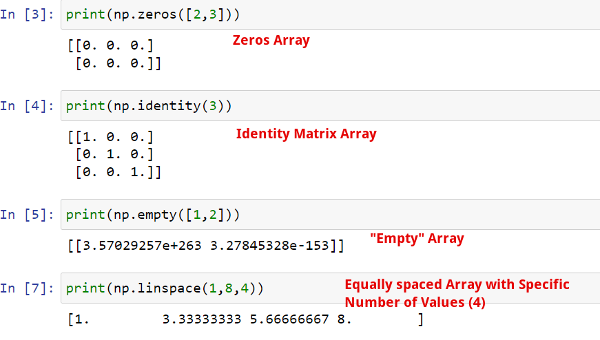
Note: You cannot generate an empty array in NumPy. Each NumPy array has a fixed, immutable size and each element in the array must be filled in when the array is created.
The np.empty() function creates the required array shape and fills it with random values. The default method creates an array of random floats.
You can create a different array datatype using the dtype parameter.
3. Array Attributes
NumPy arrays have several attributes that provide useful information about the array. Let’s look at some of them:
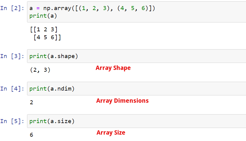
ndarray.shape: Returns the dimensions of the array as a tuple (rows, columns)
ndarray.ndim: Returns the number of dimensions in the array
ndarray.size: Returns the total number of elements in the array
ndarray.dtype: Returns the data type of the array elements
To access these attributes, use the dot notation, like so:
a = np.array([(1, 2, 3), (4, 5, 6)])

#Print out the array shape
print(a.shape)  # Output: (2, 3)
4. Data Types
NumPy provides several data types to store data in arrays, such as integer, string, float, boolean and complex. By default, NumPy tries to deduce the data type based on the input elements.
However, you can also explicitly specify the data type using the dtype keyword. For example:
import numpy as np
a = np.array([1, 2, 3], dtype=float)  # Creates an array of floats
Common NumPy data types include:
np.int32: 32-bit integer
np.int64: 64-bit integer
np.float32: 32-bit floating-point number
np.float64: 64-bit floating-point number
np.complex: Complex number, represented by two 64-bit floating-point numbers
You can also convert arrays from one data type to another. In this example, here’s how we can convert the Integer array a into a Boolean array arr using the np.array() method.
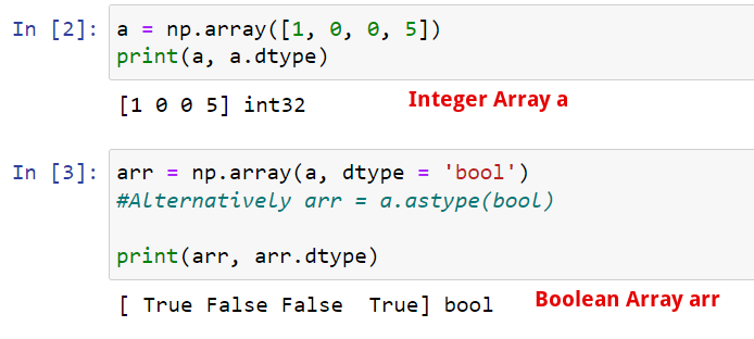
From the example, we can see the array() method converts the array elements into boolean values. These boolean values then form the new NumPy array arr.
Understanding these basic concepts of NumPy will allow you to effectively work with arrays and perform a variety of mathematical NumPy operations. For example, you can check out our video on how to transform and code addresses In Python.
In it, we used Python Pandas and NumPy data types to geocode home addresses.
Array Manipulation
In this section, you will learn about various array shape manipulation techniques in NumPy. We will discuss reshaping, concatenation, copying, splitting, adding/removing elements, indexing, and slicing.
These techniques are crucial for effectively working with array data in your data science projects.
Let’s dive into each sub-section.
1. Reshaping
Reshaping an array in NumPy is a common task you’ll perform. You might need to change the shape of your array to match the requirements of a function or an algorithm.
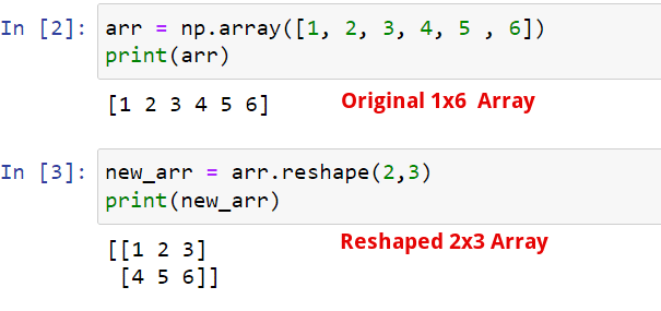
To reshape an array, use the reshape() function:
arr = np.array([1, 2, 3, 4, 5, 6])
new_arr = arr.reshape(2, 3)
This will convert your one-dimensional array into a two-dimensional array with 2 rows and 3 columns.
Note: Make sure the new shape you provide has the same size (number of array elements) as the original array.
2. Copying
You can copy the elements in one NumPy array to another using the copy() method. You should note that using the assignment operator ‘=’ creates a shallow copy.
#Creating a shallow copy of a NumPy array
a = np.array([9, 6, 12, 16, 20])
b = a
b[0] = 19

print(a) #Output:[19, 6, 12, 16, 20]
print(b) #Output:[19, 6, 12, 16, 20]
The new array only references the old array in the system’s memory. They contain the same elements and they are not independent of each other.
By using the deep copy, you create a new NumPy array that contains the same data as the old one while being independent of it.
#Creating a deep copy of a NumPy array
a = np.array([9, 6, 12, 16, 20])
b = np.copy(a)
b[0] = 19

print(a) #Output:[9, 6, 12, 16, 20]
print(b) #Output:[19, 6, 12, 16, 20]
3. Concatenation
Occasionally, you may need to merge two arrays into a single one. In NumPy, you can use the concatenate() function to join arrays along an existing axis:
import numpy as np

arr1 = np.array([1, 2, 3])
arr2 = np.array([4, 5, 6])
result = np.concatenate((arr1, arr2))
This combines arr1 and arr2 into a single array. Keep in mind that the arrays being concatenated should have the same shape, except along the specified axis.
4. Splitting
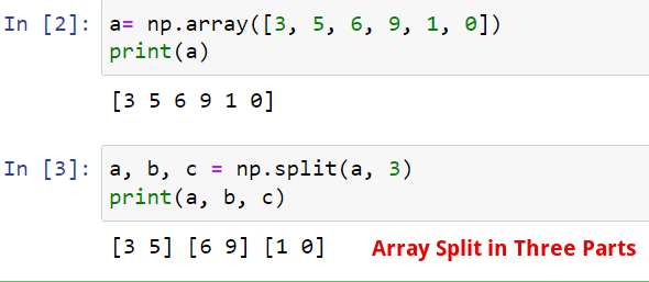
Splitting is the opposite of concatenation. You can divide an array into smaller sub-arrays using the split() function:
arr = np.array([1, 2, 3, 4, 5, 6])
result = np.split(arr, 3)
This splits the array into 3 equal-sized sub-arrays. Ensure that the number of splits you specify can evenly divide the size of the array along the given axis.
5. Adding/Removing Elements
Adding or removing elements in a NumPy array can be achieved using the append() and delete() functions. You can use the former to append values to the end of the array while the latter deletes the element at a specified index.
Here’s an example:
arr = np.array([1, 2, 3])

arr = np.append(arr, [4, 5, 6]) # Appends values to the end of the array
arr = np.delete(arr, 0) # Removes the array element on index 0
Keep in mind that NumPy arrays have a fixed size. When using append() or delete(), a new array is created, and the original one is not modified.
6. Indexing
You can perform indexing operations on NumPy arrays the same way you’d do them on Python lists or tuples. Let’s look at how you can access or change array elements in a given array.
arr = np.array([1, 2, 3])

#Returns the array element on index 1
element_2 = b[1]

#Change the array element on index 0
arr[0]= 89
7. Slicing
You can also slice NumPy arrays to extract or view a section of the data the same way you’d do Python lists or sets. Let’s take a look at an example below:
arr1 = np.array([1, 2, 3, 4, 5, 6, 7])
arr2 = np.array([(1, 2, 3, 6, 0), (4, 5, 6, 11, 13)])

# To return the first 3 elements of arr1
print(arr1[0:3]) #Output: [1, 2, 3]

# To return the second row in arr2
b = arr2[1, : ].copy() #Output: [4, 5, 6, 11, 13]
Note: Slicing creates a shallow copy that still references the main array. So, any change you make to the sliced data will be applied to the main array and vice versa.
To avoid this, you can use the copy() method to create a deep, independent copy.
Elementary Functions
In this section, you’ll learn about different elementary functions in NumPy, which will ease your data analysis tasks. We’ll cover arithmetic operations, trigonometry, and exponents and logarithms.
1. Arithmetic Operations
NumPy offers various math operations on arrays that make them simple and efficient to work with. array mathematics vector math
Some of the operations are:
Addition: numpy.add(x1, x2)
Subtraction: numpy.subtract(x1, x2)
Multiplication: numpy.multiply(x1, x2)
Division: numpy.divide(x1, x2)
Modulus: numpy.mod(x1, x2)
Power: numpy.power(x1, x2)
Square root: numpy.sqrt(x)
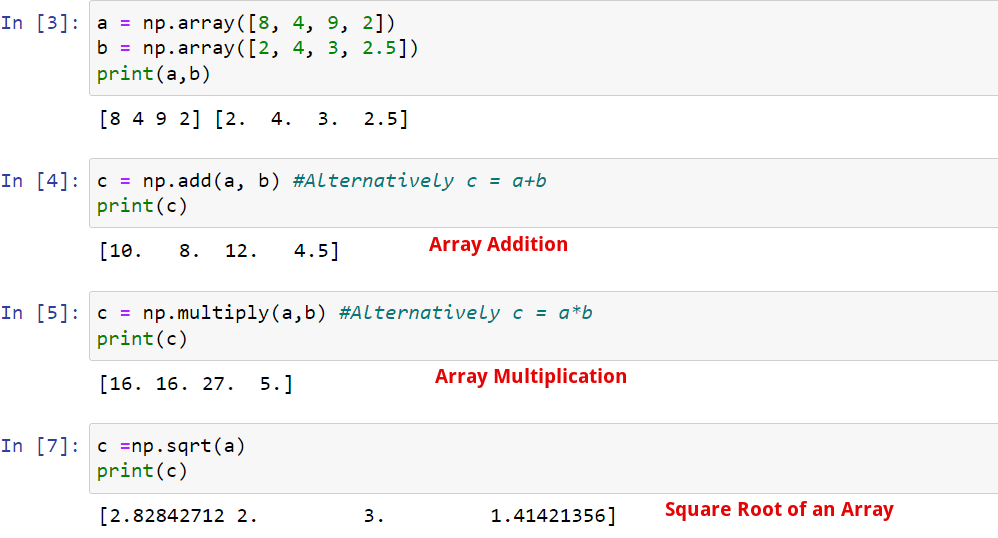
Note: When using these operations, the two arrays must be the same shape. If not, you’ll run into errors.
There is an exception for certain arrays thanks to a NumPy feature called broadcasting. We’ll cover that in a later section.
You can perform these operations element-wise on the arrays, which makes them highly efficient for large-scale data manipulation.
2. Trigonometry
Trigonometric functions play a significant role in various mathematical and scientific computations. NumPy provides a wide range of trigonometric functions.
Some of the essential functions are:
Sine: numpy.sin(x)
Cosine: numpy.cos(x)
Tangent: numpy.tan(x)
Arcsine: numpy.arcsin(x)
Arccosine: numpy.arccos(x)
Arctangent: numpy.arctan(x)
These functions work seamlessly with arrays, making it easier for you to perform vectorized computations on large datasets.
3. Exponents and Logarithms
Exponents and logarithms are crucial for various numerical operations. NumPy provides an extensive collection of functions for dealing with exponents and logarithms.
Some of the primary functions are:
Exponential: numpy.exp(x)
Logarithm(base e): numpy.log(x)
Logarithm(base 10): numpy.log10(x)
Logarithm(base 2): numpy.log2(x)
Utilizing these functions, you can quickly perform complex mathematical operations on each element in the array. This makes your data analysis tasks more accessible and efficient.
Array Analysis
In this section, we will discuss various techniques to analyze arrays and array elements in NumPy. Some of the key features we will cover include aggregate functions, statistical functions, searching, and sorting.
1. Aggregate Functions
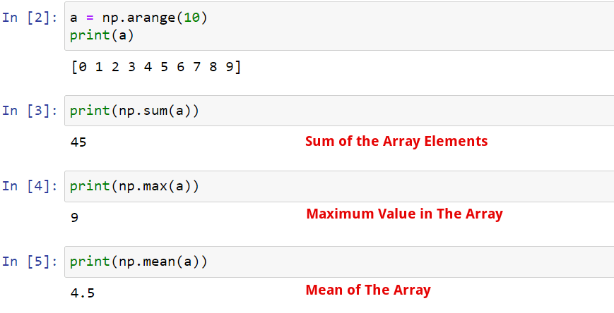
NumPy provides several aggregate functions that allow you to perform operations on arrays, such as summing all their elements, finding the minimum or maximum value, and more:
sum: np.sum(your_array) – Calculate the sum of all the elements in the array.
min: np.min(your_array) – Find the minimum array element.
max: np.max(your_array) – Find the maximum array element.
mean: np.mean(your_array) – Calculate the mean of the values in the array.
median: np.median(your_array) – Find the median of the values in the array.
2. Statistical Functions
NumPy also has a variety of statistical functions to help you analyze data:
std: np.std(your_array) – Calculate the standard deviation of the values in the array.
var: np.var(your_array) – Calculate the variance of the values in the array.
corrcoef: np.corrcoef(your_array) – Calculate the correlation coefficient of the array.
3. Searching
Searching in NumPy arrays can be done using various methods:
argmin: np.argmin(your_array) – Find the index of the minimum array element.
argmax: np.argmax(your_array) – Find the index of the maximum array element.
where: np.where(condition) – Return the indices of elements in the array that satisfy the given condition.
4. Sorting
You can sort the elements in your array using the following functions:
sort: np.sort(your_array) – Sort the elements in the array in ascending order.
argsort: np.argsort(your_array) – Returns the indices that would sort the array.
With these functions and techniques, you can conveniently analyze and manipulate your NumPy arrays to uncover valuable insights and support your data analysis efforts.
Advanced Functions
In this section, we’ll explore some advanced functions in NumPy to help you work more efficiently with your data. We’ll cover the Broadcasting and Linear Algebra functions.
1. Broadcasting
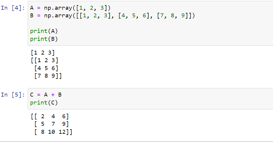
Broadcasting is a powerful NumPy feature that allows you to perform operations on arrays with different shapes and sizes. It works by automatically expanding the dimensions of the smaller array to match the larger array, making it easier to perform element-wise operations.
Here’s an example:
import numpy as np
A = np.array([1, 2, 3])
B = np.array([[1, 2, 3], [4, 5, 6], [7, 8, 9]])

C = A + B
In this example, the 1D array A is broadcasted to match the shape of the 2D array B, allowing element-wise addition.
Keep these rules in mind when working with broadcasting:
The dimensions of the arrays must be compatible (either the same size or one of them is 1).
Broadcasting is applied from the trailing dimensions and works towards the leading dimensions.
2. Linear Algebra
NumPy provides several linear algebra functions that can be useful when working with multidimensional arrays. Some of these functions include:
np.dot(A, B): Computes the dot product of two arrays.
np.linalg.inv(A): Computes the inverse of a square matrix.
np.linalg.eig(A): Computes the eigenvalues and eigenvectors of a square matrix.
np.linalg.solve(A, B): Solves a linear system of equations, where A is the coefficient matrix and B is the constant matrix.
Remember to always check if your matrices are compatible before performing these operations.
Input and Output
In this section, we’ll explore how to save and load arrays, as well as how to read and write files using NumPy.
1. Saving and Loading Arrays
To save an array, you can use NumPy’s np.save() function. This function takes the filename and the array as its two main arguments.
import numpy as np
arr = np.array([1, 2, 3])

np.save('my_array.npy', arr)
To load the saved array, use the np.load() function, providing the filename as the argument.
loaded_array = np.load('my_array.npy')

print(loaded_array)
# Output: array([1, 2, 3])
You can also save and load multiple arrays using the np.save() and np.load() functions.
2. Reading and Writing to Text Files
NumPy provides functions to read and write text files with arrays, such as np.loadtxt() and np.savetxt(). You can use these functions to save and load data from file formats like a txt or CSV file.
To read a text file into an array, use the np.loadtxt() function. It takes the filename as its main argument and also supports optional arguments for specifying delimiter, dtype, and more.
arr_from_txt = np.loadtxt('data.txt', delimiter=',')
print(arr_from_txt)
To read the data from a CSV file, you can also use the np.loadtxt() function. However, make sure the delimiter is always set to the comma, “,“.
To write an array to a text file, use the np.savetxt() function. This function takes the filename and the array as its two main arguments, followed by optional arguments, such as delimiter and header.
arr_to_txt = np.array([[1, 2, 3], [4, 5, 6]])
np.savetxt('output_data.txt', arr_to_txt, delimiter=',')
These input and output functions allow you to efficiently work with arrays and text files in your data processing and manipulation tasks using NumPy.
Download Your Cheat Sheet Below
Final Thoughts
Well, that’s all you need to know to get started with the Numpy Python library! You can also use the Python Numpy cheat sheet as a handy reference when working with the library.
For more advanced features, you can check out the NumPy documentation. You can also check out this fun Python Cheat sheet we put together for both new and experienced developers.
Good Luck!


