
Compound interest is a powerful concept in the world of finance, and being able to calculate it is an important skill.
Fortunately, Microsoft Excel makes it easy to do just that.
In Excel, you can calculate compound interest using the following formula:

=P*((1+(k/m))^(m*n))
Where:
P is the principal amount
k is the nominal interest rate per annum (annual rate)
m is the number of compounding periods per annum (Compounding frequency)
n is the number of periods
Confused? Don’t worry; in this article, we’ll show you visually how to calculate compound interest step-by-step with Excel using the best financial functions available.

Excel Functions for Compound Interest
Excel provides a number of built-in functions that allow you to easily find and calculate interest on a compounding basis.
Here are the top 3 functions explained:
1. FV Function
The FV function is used to calculate the future value of an investment or loan based on a constant interest rate and periodic payments. It is helpful in determining the total amount that will be accumulated or owed at the end of the investment or loan term.

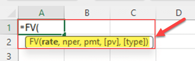
The syntax for the FV function is:
FV(rate,nper,pmt,[pv],[type])
Where:
Rate is the interest rate per period.
Nper is the total number of payment periods.
Pmt is the payment made each period and is optional.
Pv is the present value, or the principal value.
Type is a value indicating when payments are due (0 for the end of the period or 1 for the beginning).
The FV function is particularly useful when you want to find the future value of a series of regular payments, like a monthly deposit in a savings account or the regular payments on a loan.
Let’s say you’ve put $1,000 into a personal finance investment for three years, and it’s earning a 6% interest rate with compounding. You can find compound interest using the below formula.
=FV(Rate,Nper,,-Pv)-Pv
2. PV Function
The PV function in Excel is used to calculate the present value of an investment or loan, based on a constant interest rate and a series of periodic payments. It is a helpful tool for determining the initial amount required to achieve a desired future value.
The syntax for the PV function is:
PV(rate, nper, pmt, [fv], [type])
Where the arguments are:
Rate is the interest rate per period.
Nper is the total number of payment periods.
Pmt is the payment made each period and is optional.
Fv is the future value, or the desired amount at the end of the investment or loan term.
Type is a value indicating when payments are due (0 for the end of the period or 1 for the beginning).
The PV function is particularly useful when you want to calculate the present value of a series of regular payments, like the future value of a savings account or the future value of a loan.
Now, assume that your investment has grown to $1,191.02 after 3 years at a 6% p.a compounding interest rate. You can find previously accumulated interest using the below Excel compound interest formula.
=Fv-PV(Rate,Nper,,-Fv)
Remember to enter fv argument of the PV function as a negative value.
3. EFFECT Function
The EFFECT function in Microsoft Excel is utilized to calculate the effective annual interest rate, also known as the annual equivalent rate (AER) or the annual percentage rate (APR). The effective interest rate is the interest rate on a loan or financial product expressed on an annualized basis, considering the effect of compounding within a given period.

The syntax for the EFFECT function is as follows:
=EFFECT(nominal_rate, npery)
Where:
nominal_rate: This is the nominal interest rate per period, usually expressed as a percentage.
npery: This represents the number of compounding periods per year.
The EFFECT function is particularly useful when you need to determine the true annual interest rate that incorporates the impact of compounding. This is crucial in understanding the actual cost of a loan or the true return on an investment, especially when interest is compounded more frequently than once a year.
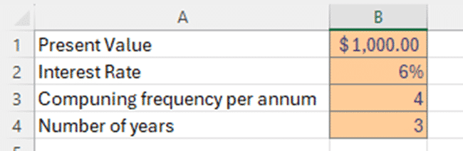
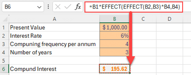
Assume that you have invested $1,000 for 3 years on 6% interest rate compounded quarterly. You can find compound interest using the below formula.
=P+(P*EFFECT(EFFECT(k,m)*n,n))
Where:
P is the principal amount
k is the nominal interest rate per annum (annual rate)
m is the number of compounding periods per annum (Compounding frequency)
n is the number of periods
Using the Power Formula to Calculate Compound Interest
Excel offers a range of financial functions that can be utilized to calculate compound interest. However, if you prefer, you can also find compound interest using a simple formula with Excel’s power function.
Here’s a step-by-step guide to using the power function to calculate interest earned on a compounded basis:
Step 1: Understand the Formula
The formula for calculating compound interest is:
A=P*((1+(k/m))^(m*n))
Where:
A = the future value of the investment/loan, including interest
P = the principal investment amount (the initial deposit or loan amount)
k = the annual interest rate (decimal)
m = the number of times that interest is compounded per year
n = the time the money is invested or borrowed for, in years
Step 2: Organize Your Data
In Excel, you can organize the data used in the formula in separate cells, making it easier to get compound interest.
For example, you could organize the data as follows:
Cell B1: Initial investment amount
Cell B2: Annual interest rate
Cell B3: Number of times the interest is compounded per year
Cell B4: Number of years the investment is held
You can then use these cells in your compound interest formula, which makes it easier to adjust the variables if needed.
Step 3: Calculate the Compound Interest
To calculate the compound interest, use the formula =P(1+r/n)^(n*t)-P in a blank cell, where P is the principal investment amount and r, n, and t are the variables described above. For example, if you have your principal amount in cell B1, the formula would be:
=B1*((1+B2/B3)^(B4*B4))-B1
Step 4: Evaluate the Results
Once you have calculated the compound interest, you can easily evaluate the results and make adjustments if necessary.
For example, you can change the annual interest rate, the number of times the interest is compounded per year, or the number of years the investment is held to see how it affects the compound interest.
By using the power function in Excel to find compound interest, you can easily apply the compound interest formula to your financial data, make adjustments as needed, and evaluate the results.

Final Thoughts
Understanding how to calculate compound interest in Excel is a valuable skill that can be applied to various financial scenarios.
By using the FV, PV, and EFFECT functions, you can quickly and accurately calculate the future value, present value, and effective interest rate needed for an investment or loan.
Furthermore, these functions allow you to input key variables, such as the interest rate, payment amounts, and payment periods, to obtain a clear picture of the financial outcomes.
Additionally, utilizing the power function enables you to perform compound interest calculations without relying solely on built-in Excel functions.
Ready to learn more than Excel and take your data skills to the next level?
Explore cutting-edge developments in Power BI & Power Platform at the “Innovations In Power BI & Power Platform Summit” events.
The video below provides insights into sessions ranging from beginner to advanced, covering a variety of data analytics and innovations.
Frequently Asked Questions
How can you calculate compound interest using Excel formulas?
In Excel, you can calculate compound interest using the formula:
=P*((1+(k/m))^(m*n))
Where:
P is the principal amount
k is the nominal interest rate per annum
m is the number of compounding periods per annum
n is the number of periods
This formula will give you the future value of the investment.
What Excel functions are available for compound interest calculations?
Excel provides several functions for compound interest calculations, including:
FV: Used to determine the future value of an investment
PV: Used to determine the present value of an investment
EFFECT: Used to determine the effective annual interest rate, considering compounding over a specified number of periods.
RATE: Used to determine the interest rate required to achieve a specific investment amount
Can Excel calculate compound interest with additional contributions?
Yes, Excel can calculate compound interest with additional contributions. You can use the FV function and include the PMT argument for periodic contributions.
The formula would be:
=FV(rate, nper, pmt, pv)
Where:
rate is the interest rate per period
nper is the total number of periods
pmt is the periodic payment
pv is the initial investment amount
How can you use the power function to calculate compound interest in Excel?
To calculate compound interest using the power function, you can use the formula:
=P((1+(k/m))^(m*n))
This formula will give you the future value of the investment, where P is the principal amount, k is the interest rate per period, m stands for compounding frequency and n is the number of periods.
What is the future value of an investment with compound interest?
The future value of an investment with compound interest can be calculated using the formula:
FV = P*(1+r)^n
Where:
FV is the future value
P is the principal amount
r is the interest rate per period
n is the number of periods
This formula takes into account the effect of compounding, where the interest is added to the principal amount, and subsequent interest is then calculated on the new total.
How do you calculate the present value of an investment with compound interest in Excel?
To calculate the present value of an investment with compound interest in Excel, you can use the PV function.
The formula is:
PV = PV(rate, nper, pmt, fv)
Where:
rate is the interest rate per period
nper is the total number of periods
pmt is the periodic payment
fv is the future value


